Big O Constant, linear, quadratic, logarithmic, and exponential. math · complexity Study sequence: [Vectors](vectors.html) · [Matrices](matrices.html) · [Matrix applications](matrix-applications.html) · [Calculus](calculus.html) · Big O · [Geometry](geometry.html) · [Signals](signals.html) · [Neural nets](neural-nets.html) · [Distributions](distributions.html) ## Constant Complexity, $O(1)$ The output rate remains the same. $O(1)$ means the work stays a constant. One more input adds no work, so the graph is a flat line. ```python def mlplot( x, y, title="", annotation=None, anotx=50, anoty=1.001, anoax=50, anoay=1.03, anosize='x-small', xlab="input", ylab="output", size=(8,7), filename=None, logox=98, logoy=.946 ): plt.figure(facecolor='#000000',edgecolor='#000000',figsize=size,layout='tight') plt.axes(facecolor='#000000') plt.tick_params(colors='white', grid_color='white') plt.xticks(fontfamily='monospace', fontsize='small',fontstyle='italic', fontweight='semibold') plt.yticks(fontfamily='monospace', fontsize='small',fontstyle='italic', fontweight='semibold') plt.title(title, fontfamily='monospace', fontsize='medium', fontstyle='italic', fontweight='semibold', color='#ffffff') if annotation is not None: plt.annotate(annotation,(anotx, anoty), (anoax,anoay), arrowprops={'arrowstyle':'-|>','color':'#ffffff'}, color='#ffffff', fontfamily='monospace', fontsize=anosize,fontstyle='italic', fontweight='semibold') plt.xlabel(xlab, loc='left', fontfamily='monospace', fontsize='small',fontstyle='italic', fontweight='semibold', color='#ffffff') plt.ylabel(ylab, loc='bottom', fontfamily='monospace', fontsize='small', fontstyle='italic', fontweight='semibold', color='#ffffff') mpl.rc('axes', edgecolor='white', facecolor='white') plt.text(logox,logoy,'machine-labs.io',fontfamily='monospace', fontsize='xx-small',fontstyle='italic', fontweight='semibold', color='#ffffff') plt.plot(x,y,color='#ffffff'); if filename is not None: plt.savefig(filename, metadata={'title':f'{filename}','author':'machine-labs.io'}) x = [i for i in range(100)] y = [1 for i in range(100)] mlplot(x,y, annotation='The output rate remains the same.', title='Constant Complexity, $O(1)$', size=(8,7), logox=90, filename='constant', xlab='The length of an input.', ylab='The rate of output growth.' # check my language here ) ``` 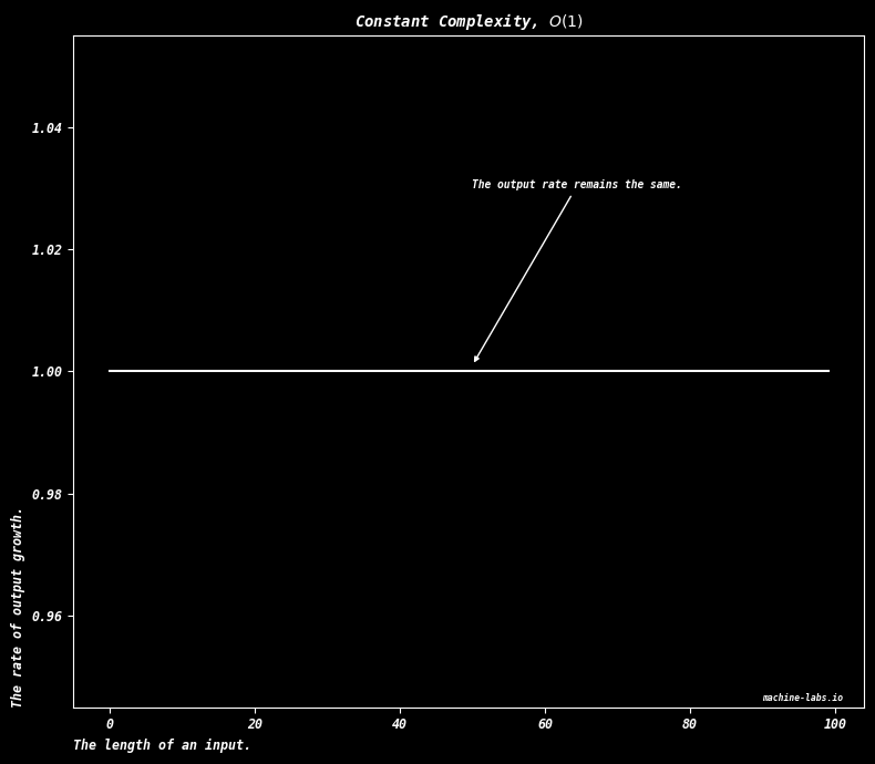 ## Linear Complexity, $O(n)$ As the input size increases, the output rate increases, at the same rate. $O(n)$ means the work grows in proportion to $n$, the length of the input. Double the input and the work doubles, so the graph is a straight line through the origin. ```python def mlplot( x, y, title="", annotation=None, anotx=40, anoty=42, anoax=20, anoay=80, anosize='x-small', xlab="input", ylab="output", size=(8,7), filename=None, logox=98, logoy=-4 ): plt.figure(facecolor='#000000',edgecolor='#000000',figsize=size,layout='tight') plt.axes(facecolor='#000000') plt.tick_params(colors='white', grid_color='white') plt.xticks(fontfamily='monospace', fontsize='small',fontstyle='italic', fontweight='semibold') plt.yticks(fontfamily='monospace', fontsize='small',fontstyle='italic', fontweight='semibold') plt.title(title, fontfamily='monospace', fontsize='medium', fontstyle='italic', fontweight='semibold', color='#ffffff') if annotation is not None: plt.annotate(annotation,(anotx, anoty), (anoax,anoay), arrowprops={'arrowstyle':'-|>','color':'#ffffff'}, color='#ffffff', fontfamily='monospace', fontsize=anosize,fontstyle='italic', fontweight='semibold') plt.xlabel(xlab, loc='left', fontfamily='monospace', fontsize='small',fontstyle='italic', fontweight='semibold', color='#ffffff') plt.ylabel(ylab, loc='bottom', fontfamily='monospace', fontsize='small', fontstyle='italic', fontweight='semibold', color='#ffffff') mpl.rc('axes', edgecolor='white', facecolor='white') plt.text(logox,logoy,'machine-labs.io',fontfamily='monospace', fontsize='xx-small',fontstyle='italic', fontweight='semibold', color='#ffffff') plt.plot(x,y,color='#ffffff'); if filename is not None: plt.savefig(filename, metadata={'title':f'{filename}','author':'machine-labs.io'}) # O(n) def lin(n): _ = 0 for i in range(n): _+=1 return (n,_) x=[] y=[] for i in range(100): x.append(lin(i)[0]) y.append(lin(i)[1]) mlplot(x,y, annotation='As the input size increases,\nthe output rate increases,\nat the same rate.', title='Linear Complexity, $O(n)$', size=(8,7), logox=90, filename='linear', xlab='The length of an input.', ylab='The rate of output growth.' # check my language here ) ``` 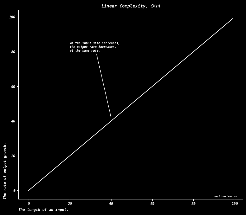 ## Quadratic Complexity, $O(n^2)$ As the input size increases, the output rate increases, at the input rate squared. $O(n^2)$ means the work grows with the square of $n$. Double the input and the work is multiplied by four. The nested loops below each run $n$ times, so the inner step runs $n\times n$ times. ```python def mlplot( x, y, title="", annotation=None, anotx=40, anoty=2000, anoax=10, anoay=8500, anosize='x-small', xlab="input", ylab="output", size=(8,7), filename=None, logox=92, logoy=-400 ): plt.figure(facecolor='#000000',edgecolor='#000000',figsize=size,layout='tight') plt.axes(facecolor='#000000') plt.tick_params(colors='white', grid_color='white') plt.xticks(fontfamily='monospace', fontsize='small',fontstyle='italic', fontweight='semibold') plt.yticks(fontfamily='monospace', fontsize='small',fontstyle='italic', fontweight='semibold') plt.title(title, fontfamily='monospace', fontsize='medium', fontstyle='italic', fontweight='semibold', color='#ffffff') if annotation is not None: plt.annotate(annotation,(anotx, anoty), (anoax,anoay), arrowprops={'arrowstyle':'-|>','color':'#ffffff'}, color='#ffffff', fontfamily='monospace', fontsize=anosize,fontstyle='italic', fontweight='semibold') plt.xlabel(xlab, loc='left', fontfamily='monospace', fontsize='small',fontstyle='italic', fontweight='semibold', color='#ffffff') plt.ylabel(ylab, loc='bottom', fontfamily='monospace', fontsize='small', fontstyle='italic', fontweight='semibold', color='#ffffff') mpl.rc('axes', edgecolor='white', facecolor='white') plt.text(logox,logoy,'machine-labs.io',fontfamily='monospace', fontsize='xx-small',fontstyle='italic', fontweight='semibold', color='#ffffff') plt.plot(x,y,color='#ffffff'); if filename is not None: plt.savefig(filename, metadata={'title':f'{filename}','author':'machine-labs.io'}) # O(n^2) generate input # two nested for loops # that take n as the input # means we process n*n # values. n^2. def square(n): y = 0 for i in range(n): # these two for loops take for j in range(n): # an input as the range y+=1 return (n,y) x=[] y=[] for i in range(100): x.append(square(i)[0]) y.append(square(i)[1]) mlplot(x,y, annotation='As the input size increases,\nthe output rate increases,\nat the input rate squared.', title='Quadratic Complexity, $O(n^2)$', size=(8,7), logox=90, filename='quadratic', xlab='The length of an array.', ylab='The rate of output growth.' # check my language here ) ``` 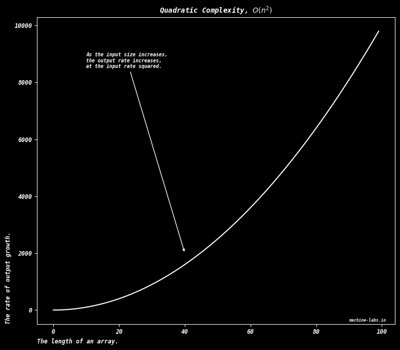 ## Logarithmic Complexity, $O(\log n)$ As the input size increases the output rate decreases at the logarithm of the input. A logarithm is the count of how many times you can divide $n$ by a fixed fraction, often 2, before you reach 1. $O(\log n)$ names work that grows like that count. The code plots $\log n$, the natural logarithm, whose base is $e$, about 2.718. ```python def mlplot( x, y, title="", annotation=None, anotx=22, anoty=3, anoax=60, anoay=.5, anosize='x-small', xlab="input", ylab="output", size=(8,7), filename=None, logox=98, logoy=-.2 ): plt.figure(facecolor='#000000',edgecolor='#000000',figsize=size,layout='tight') plt.axes(facecolor='#000000') plt.tick_params(colors='white', grid_color='white') plt.xticks(fontfamily='monospace', fontsize='small',fontstyle='italic', fontweight='semibold') plt.yticks(fontfamily='monospace', fontsize='small',fontstyle='italic', fontweight='semibold') plt.title(title, fontfamily='monospace', fontsize='medium', fontstyle='italic', fontweight='semibold', color='#ffffff') if annotation is not None: plt.annotate(annotation,(anotx, anoty), (anoax,anoay), arrowprops={'arrowstyle':'-|>','color':'#ffffff'}, color='#ffffff', fontfamily='monospace', fontsize=anosize,fontstyle='italic', fontweight='semibold') plt.xlabel(xlab, loc='left', fontfamily='monospace', fontsize='small',fontstyle='italic', fontweight='semibold', color='#ffffff') plt.ylabel(ylab, loc='bottom', fontfamily='monospace', fontsize='small', fontstyle='italic', fontweight='semibold', color='#ffffff') mpl.rc('axes', edgecolor='white', facecolor='white') plt.text(logox,logoy,'machine-labs.io',fontfamily='monospace', fontsize='xx-small',fontstyle='italic', fontweight='semibold', color='#ffffff') plt.plot(x,y,color='#ffffff'); if filename is not None: plt.savefig(filename, metadata={'title':f'{filename}','author':'machine-labs.io'}) def log(n): import math y = 0 for i in range(n): y = math.log(n) x=[] y=[] for i in range(1, 100): x.append(i) y.append(math.log(i)) mlplot(x,y, annotation='As the input size increases\nthe output rate decreases\nat the logarithm of the input.', title='Logarithmic Complexity, $O(log\ n)$', size=(8,7), logox=90, filename='logarithmic', xlab='The length of an input.', ylab='The rate of output growth.' # check my language here ) ``` 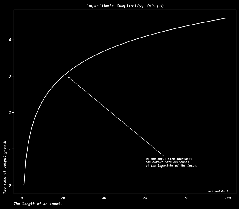 ## Exponential Complexity, $O(2^n)$ $O(2^n)$ means each new input doubles the work. Exponential growth is a constant raised to the input. Here the constant is 2, so the plotted values are $2^n$. The vertical axis of this figure is itself on a log scale, equal steps meaning equal multiplications, which is why a doubling curve can be drawn in the window. ```python def mlplot( x, y, title="", annotation=None, anotx=50, anoty=1.001, anoax=50, anoay=1.03, anosize='x-small', xlab="input", ylab="output", size=(8,7), filename=None, logox=98, logoy=.946 ): plt.figure(facecolor='#000000',edgecolor='#000000',figsize=size,layout='tight') plt.axes(facecolor='#000000') plt.tick_params(colors='white', grid_color='white') plt.xticks(fontfamily='monospace', fontsize='small',fontstyle='italic', fontweight='semibold') plt.yticks(fontfamily='monospace', fontsize='small',fontstyle='italic', fontweight='semibold') plt.title(title, fontfamily='monospace', fontsize='medium', fontstyle='italic', fontweight='semibold', color='#ffffff') if annotation is not None: plt.annotate(annotation,(anotx, anoty), (anoax,anoay), arrowprops={'arrowstyle':'-|>','color':'#ffffff'}, color='#ffffff', fontfamily='monospace', fontsize=anosize,fontstyle='italic', fontweight='semibold') plt.xlabel(xlab, loc='left', fontfamily='monospace', fontsize='small',fontstyle='italic', fontweight='semibold', color='#ffffff') plt.ylabel(ylab, loc='bottom', fontfamily='monospace', fontsize='small', fontstyle='italic', fontweight='semibold', color='#ffffff') plt.yscale('log', base=10) mpl.rc('axes', edgecolor='white', facecolor='white') plt.text(logox,logoy,'machine-labs.io',fontfamily='monospace', fontsize='xx-small',fontstyle='italic', fontweight='semibold', color='#ffffff') plt.plot(x,y,color='#ffffff'); if filename is not None: plt.savefig(filename, metadata={'title':f'{filename}','author':'machine-labs.io'}) # O(n) def lin(n): _ = 0 for i in range(n): _+=1 return (n,_) x=[] y=[] for i in range(100): x.append(lin(i)[0]) y.append(2**i) mlplot(x,y, # annotation='The output rate remains the same.', title='Exponential Complexity, $O(2^n)$', size=(8,7), logox=10, filename='exponential', xlab='The length of an input.', ylab='The rate of output growth.' # check my language here ) ``` 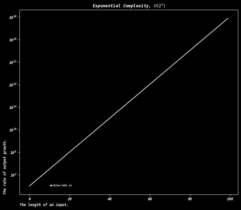 Put on one picture, the constant grows slowest, then the logarithm, then the straight line, then the square, then the exponential. The same shapes, plus $n\log n$ and the factorial, are compared as vectors in [Vectors](vectors.html#pearson-correlation-coefficient). Next: [Geometry](geometry.html).