Calculus A derivative measures how a function changes as its input changes. math · calculus Study sequence: [Vectors](vectors.html) · [Matrices](matrices.html) · [Matrix applications](matrix-applications.html) · Calculus · [Big O](big-o.html) · [Geometry](geometry.html) · [Signals](signals.html) · [Neural nets](neural-nets.html) · [Distributions](distributions.html) # Limits ## Simple A limit is defined as $\lim_{x \to a} f(x)$ Specifically, $\lim_{x \to 2} x^2 = 4$ y = x**2 ```python def square(x): return x**2 linspace = np.linspace(0,2,100) y = [square(x) for x in linspace] plt.plot(linspace,y) ``` 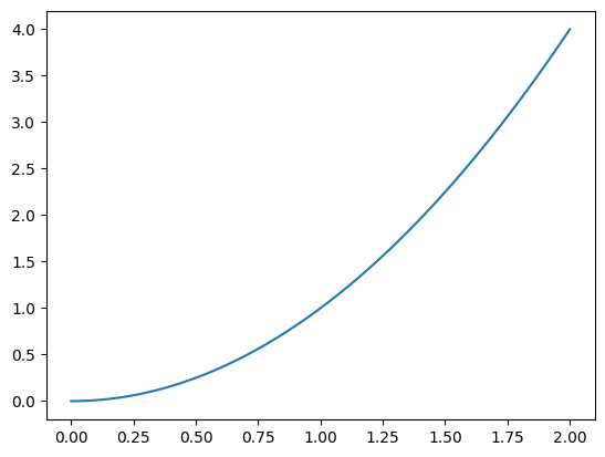 # The Concept of Derivative A **derivative** is one of the main ideas in calculus that measures how a function changes as its input changes. It can be viewed as an instantaneous rate of change or slope at any point on the graph of the function. This concept is fundamental to understanding many phenomena, from physics and engineering to economics. The slope is the change in the output divided by the change in the input. Let $\Delta x$ be a small step in the input. The difference quotient is that ratio, and the derivative is the value the ratio approaches as the step shrinks toward zero: $$f'(x)=\lim_{\Delta x\to 0}\frac{f(x+\Delta x)-f(x)}{\Delta x}$$ A limit is the number an expression settles toward. The section on $1/x$ below carries this definition through one function. Considering our functions $$f(x) = 2*x^3 - 5*x + 7$$ and its derivative $$f'(x) = df/dx = 6*x^2 - 5$$ - The function **f(x)** represents a curve on the graph. At any point along this curve, you can imagine drawing a tangent (a line that just 'touches' the curve at that point). The slope of that tangent line is what we call the derivative at that particular point. - The function **f'(x)** represents another curve, which shows how fast or slow the original curve (f(x)) is changing at any given x value. If you follow a point along this f'(x) curve from left to right, it's like watching how the slope of our tangent line on the f(x) plot changes - that's exactly what the derivative tells us! f(x) = 2*x^3 - 5*x + 7 ```python import matplotlib.pyplot as plt import numpy as np # Define the functions def f(x): return 2*x**3 - 5*x + 7 def df(x): return 6*x**2 - 5 # Create an array of x values from -10 to 10 x = np.linspace(-10, 10, 400) y = f(x) dy = df(x) plt.figure(figsize=(12,5)) # Plot the function f(x) and its derivative df(x) plt.subplot(1,2,1) # 1 row, 2 columns, first plot plt.plot(x, y) plt.title('f(x) = 2*x^3 - 5*x + 7') plt.grid() plt.subplot(1,2,2) # 1 row, 2 columns, second plot plt.plot(x, dy) plt.title('f\'(x) = df/dx = 6*x^2 - 5') plt.grid() # Show the plots plt.show() ``` 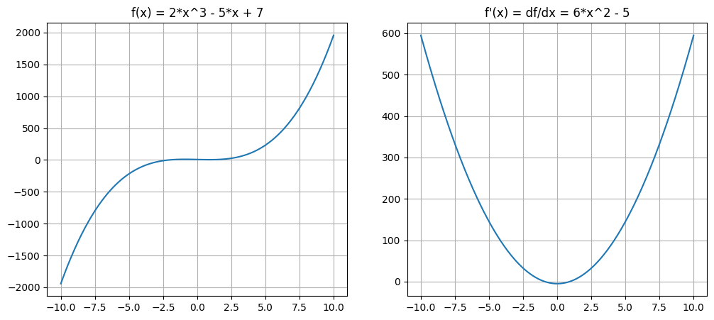 Reciprocal Function (1/x) ```python # Create data for 1/x function, avoiding x=0 x = np.linspace(-10, 10, 200) # Start from 0.1 to avoid division by zero y = 1/x # Create figure and axis plt.figure(figsize=(10, 6)) # Plot 1/x plt.plot(x, y, 'r-', label='y = 1/x') # Customize the plot plt.grid(True, alpha=0.2) plt.xlabel('x') plt.ylabel('y') plt.title('Reciprocal Function (1/x)') plt.legend() plt.show() ``` 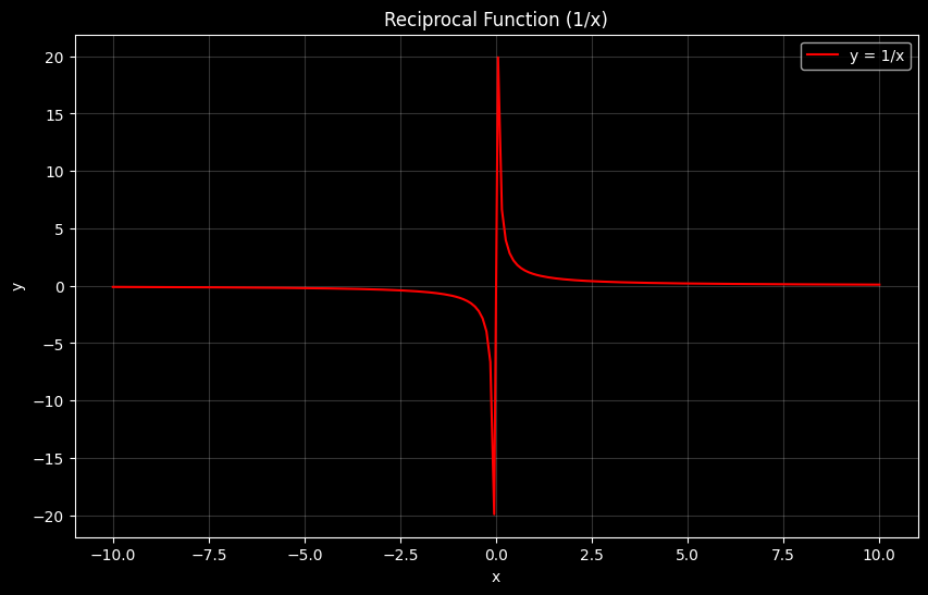 Derivative of Reciprocal Function (-1/x²) ```python # Create data for derivative of 1/x function (which is -1/x^2) x = np.linspace(-10, 10, 200) # Use same x range as original function y = -1/(x**2) # Derivative of 1/x is -1/x^2 # Create figure and axis plt.figure(figsize=(10, 6)) # Plot derivative of 1/x plt.plot(x, y, 'g-', label='y = -1/x²') # Customize the plot plt.grid(True, alpha=0.2) plt.xlabel('x') plt.ylabel('y') plt.title('Derivative of Reciprocal Function (-1/x²)') plt.legend() plt.show() ``` 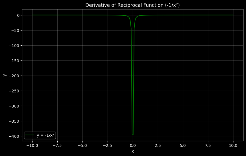 Finding the Derivative of $\frac{1}{x}$ Let's find the derivative of $f(x) = \frac{1}{x}$ using the limit definition. Start with the limit definition: $$f'(x) = \lim_{\Delta x \to 0} \frac{f(x+\Delta x) - f(x)}{\Delta x}$$ Substitute $f(x) = \frac{1}{x}$: $f(x+\Delta x) = \frac{1}{x+\Delta x}$ $f(x) = \frac{1}{x}$ So: $$f'(x) = \lim_{\Delta x \to 0} \frac{\frac{1}{x+\Delta x} - \frac{1}{x}}{\Delta x}$$ Get common denominator: To subtract fractions, multiply each by the denominator of the other: $$\frac{1}{x+\Delta x} - \frac{1}{x} = \frac{1}{x+\Delta x} \cdot \frac{x}{x} - \frac{1}{x} \cdot \frac{x+\Delta x}{x+\Delta x}$$ $$= \frac{x}{x(x+\Delta x)} - \frac{x+\Delta x}{x(x+\Delta x)}$$ $$= \frac{x-(x+\Delta x)}{x(x+\Delta x)}$$ $$= \frac{-\Delta x}{x(x+\Delta x)}$$ So now we have: $$f'(x) = \lim_{\Delta x \to 0} \frac{\frac{-\Delta x}{x(x+\Delta x)}}{\Delta x}$$ $$= \lim_{\Delta x \to 0} \frac{-\Delta x}{x^2+x\Delta x} \cdot \frac{1}{\Delta x}$$ Cancel $\Delta x$: $$= \lim_{\Delta x \to 0} \frac{-1}{x^2+x\Delta x}$$ Take limit: $$f'(x) = -\frac{1}{x^2}$$ The derivative of $\frac{1}{x}$ is $-\frac{1}{x^2}$ Position: h(t) = -5t² + 20t Velocity: h'(t) = -10t + 20 Acceleration: h''(t) = -10 Velocity is the derivative of position, how fast the height is changing. Acceleration is the derivative of velocity, how fast that speed is changing. Here the acceleration is the constant $-10$. ```python import numpy as np import matplotlib.pyplot as plt # Position: h(t) = -5t² + 20t # Velocity: h'(t) = -10t + 20 (derivative of position) # Acceleration: h''(t) = -10 (derivative of velocity) def pos(t): return (-5 * (t**2)) + (20 * t) def vel(t): return (-10 * t) + (20) def throw(t): return (pos(t), vel(t)) x = [] y = [] y2 = [] for second in np.arange(0,4,0.1): x.append(second) y.append(throw(second)[0]) plt.plot(x, y, y2) ``` 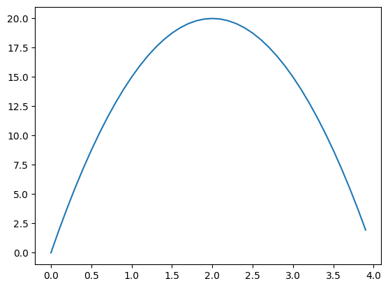 sigmoid $$\sigma(z)=\frac{1}{1+e^{-z}}$$ $e$ is about 2.718. The curve sits near 0 for a large negative input, passes through $1/2$ at $z=0$, and sits near 1 for a large positive input. Its slope is $\sigma(z)\,(1-\sigma(z))$, steepest in the middle and flat in both tails. The second derivative is the slope of that slope. The three definitions below are this curve, its slope, and that second slope. ```python def sigmoid(z): return 1 / (1 + np.exp(-z)) def sigmoid_derivative(z): s = sigmoid(z) return s * (1 - s) def sigmoid_second_derivative(z): s = sigmoid(z) return s * (1 - s) * (1 - 2*s) ``` ```python plt.plot(np.arange(-5,5,0.1), sigmoid(np.arange(-5,5,0.1))) ``` 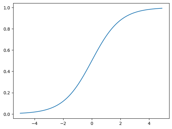 derivative of the sigmoid ```python plt.plot(np.arange(-5,5,0.1), sigmoid_derivative(np.arange(-5,5,0.1))) ``` 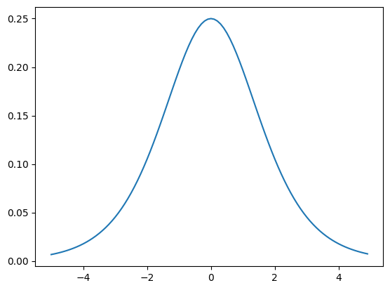 second derivative of the sigmoid ```python plt.plot(np.arange(-5,5,0.1), sigmoid_second_derivative(np.arange(-5,5,0.1))) ``` 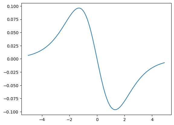 ## By hand: activation @ alan yeh. ai by hand [https://aibyhand.substack.com/](https://aibyhand.substack.com/) [https://aibyhand.substack.com/p/w4-activation](https://aibyhand.substack.com/p/w4-activation) ```python def relu(x): return np.where(x >= 0, x, x==0) def sig3(x): cond1 = x >= 2 cond2 = (-1 <= x) & (x <= 1) cond3 = (x <= -2) vals = [1, 0.5, 0] return np.select([cond1, cond2, cond3], vals) def sig5(x): cond1 = x >= 2 cond2 = (1 <= x) & (x < 2) cond3 = (0 <= x) & (x < 1) cond4 = (-2 < x) & (x < 0) cond5 = (x <= -2) vals = [1, 0.7, 0.5, 0.3, 0] return np.select([cond1, cond2, cond3, cond4, cond5], vals) def tanh3(x): cond1 = x >= 2 cond2 = (-1 <= x) & (x <= 1) cond3 = (x <= -2) vals = [1, 0, -1] return np.select([cond1, cond2, cond3], vals) def tanh5(x): cond1 = x >= 2 cond2 = (1 <= x) & (x < 2) cond3 = (0 <= x) & (x < 1) cond4 = (-2 < x) & (x < 0) cond5 = (x <= -2) vals = [1, 0.8, 0, -0.8, -1] return np.select([cond1, cond2, cond3, cond4, cond5], vals) ``` ```python relu(M([5],[4],[3],[2],[1],[0],[-1],[-2],[-3],[-4],[-5])) ``` ``` array([[5], [4], [3], [2], [1], [0], [0], [0], [0], [0], [0]]) ``` ```python relu(M([[i] for i in range(5, -6, -1)]))[0] ``` ``` array([[5], [4], [3], [2], [1], [0], [0], [0], [0], [0], [0]]) ``` ```python relu(M([2],[0],[-2])) ``` ``` array([[2], [0], [0]]) ``` ```python x=M([2],[0],[-2]) sig3(x) ``` ``` array([[1. ], [0.5], [0. ]]) ``` ```python x=M([-3],[1],[-1]) sig3(x) ``` ``` array([[0. ], [0.5], [0.5]]) ``` ```python x=M([-9],[-5],[-4]) sig3(x) ``` ``` array([[0.], [0.], [0.]]) ``` ```python x=M([11],[7],[4]) sig3(x) ``` ``` array([[1.], [1.], [1.]]) ``` ```python tanh3(M([2],[0],[-2])) ``` ``` array([[ 1], [ 0], [-1]]) ``` ```python tanh3(M([-9],[-5],[-4])) ``` ``` array([[-1], [-1], [-1]]) ``` ```python tanh3(M([11],[7],[4])) ``` ``` array([[1], [1], [1]]) ``` ```python sig3(tanh3(M([1],[2],[-3]))) ``` ``` array([[0.5], [0.5], [0.5]]) ``` ```python sig3(relu(M([1],[2],[-3]))) ``` ``` array([[0.5], [1. ], [0.5]]) ``` ```python sig5(M([0,1,-1])) ``` ``` array([[0.5, 0.7, 0.3]]) ``` ```python tanh5(M([0,1,-1])) ``` ``` array([[ 0. , 0.8, -0.8]]) ``` After a linear layer, these are in [Neural nets](neural-nets.html#by-hand-layer-then-activation). y = sin(x) ```python x = np.arange(0,10,0.1) y = np.sin(x) plt.plot(x,y) plt.grid(True, alpha=0.2) ``` 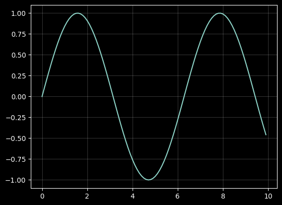 y*2, y*3, y*4, y*5 ```python x = np.arange(0,10,0.1) y = np.sin(x) plt.plot(x,y*2) plt.plot(x,y*3) plt.plot(x,y*4) plt.plot(x,y*5) plt.plot(x,y*6) plt.plot(x,y*7) plt.plot(x,y*8) plt.plot(x,y*9) plt.plot(x,y*10) plt.grid(True, alpha=0.2) ``` 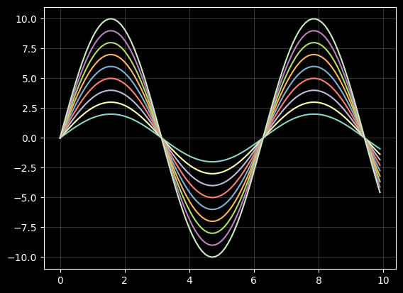 y = sin(2x) ```python x = np.arange(0,10,0.1) y = np.sin(2*x) plt.plot(x,y) plt.grid(True, alpha=0.2) ``` 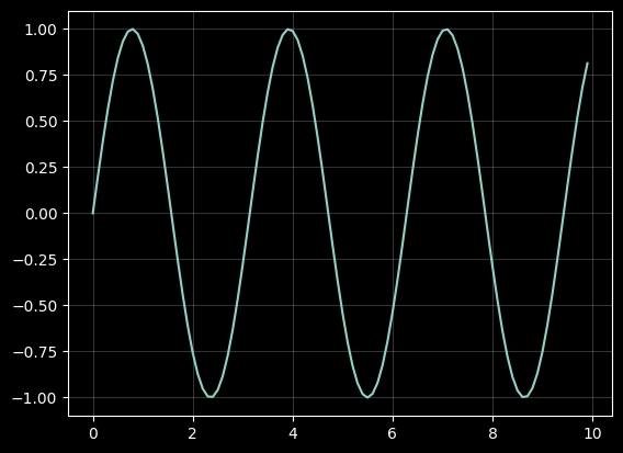 y = sin(x - 1) ```python x = np.arange(0,10,0.1) y = np.sin(x-1) plt.plot(x,y) plt.grid(True, alpha=0.2) ``` 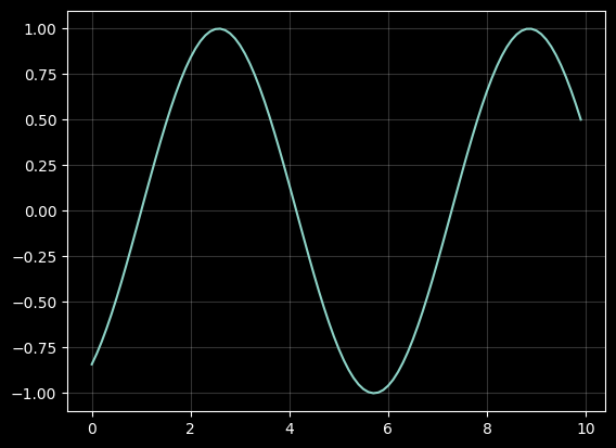 Basic sine wave ```python # Basic sine wave x = np.linspace(0, 4*np.pi, 1000) y1 = np.sin(x) # Basic y2 = 2*np.sin(x) # Amplitude = 2 y3 = np.sin(2*x) # Double frequency y4 = np.sin(x - np.pi/4) # Phase shift plt.plot(x, y1, 'b', label='Basic') plt.plot(x, y2, 'r', label='Larger A') plt.plot(x, y3, 'g', label='Higher k') plt.plot(x, y4, 'y', label='Phase shifted') plt.grid(True, alpha=0.2) plt.legend() ``` 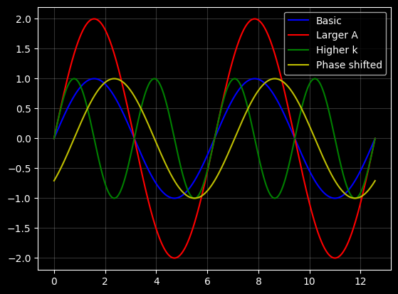 Unit Circle with Derivatives Red arrows: derivative of sin(θ) Green arrows: derivative of cos(θ) On the unit circle, the circle of radius 1, the point at angle $\theta$ is $(\cos\theta,\sin\theta)$. The radius is the straight line from the center to the point. The direction of travel along the circle is $(-\sin\theta,\cos\theta)$. Those components are the derivatives: the derivative of $\sin$ is $\cos$, and the derivative of $\cos$ is $-\sin$. ```python # Create data points for unit circle theta = np.linspace(0, 2*np.pi, 200) x = np.cos(theta) y = np.sin(theta) # Create figure and axis plt.figure(figsize=(10, 6)) # Plot unit circle plt.plot(x, y, 'b-', label='Unit Circle') # Plot arrows to show derivatives at key points # At θ=0: cos(0)=1, sin(0)=0, cos'(0)=0, sin'(0)=1 plt.arrow(1, 0, 0, 0.3, head_width=0.05, head_length=0.1, fc='r', ec='r', label="sin'(0)=1") plt.arrow(1, 0, -0.3, 0, head_width=0.05, head_length=0.1, fc='g', ec='g', label="cos'(0)=-sin(0)=0") # At θ=π/2: cos(π/2)=0, sin(π/2)=1, cos'(π/2)=-1, sin'(π/2)=0 plt.arrow(0, 1, -0.3, 0, head_width=0.05, head_length=0.1, fc='r', ec='r') plt.arrow(0, 1, 0, -0.3, head_width=0.05, head_length=0.1, fc='g', ec='g') # At θ=π: cos(π)=-1, sin(π)=0, cos'(π)=0, sin'(π)=-1 plt.arrow(-1, 0, 0, -0.3, head_width=0.05, head_length=0.1, fc='r', ec='r') plt.arrow(-1, 0, 0.3, 0, head_width=0.05, head_length=0.1, fc='g', ec='g') # At θ=3π/2: cos(3π/2)=0, sin(3π/2)=-1, cos'(3π/2)=1, sin'(3π/2)=0 plt.arrow(0, -1, 0.3, 0, head_width=0.05, head_length=0.1, fc='r', ec='r') plt.arrow(0, -1, 0, 0.3, head_width=0.05, head_length=0.1, fc='g', ec='g') # Customize the plot plt.grid(True, alpha=0.2) plt.axis('equal') plt.xlabel('cos(θ)') plt.ylabel('sin(θ)') plt.title('Unit Circle with Derivatives\nRed arrows: derivative of sin(θ)\nGreen arrows: derivative of cos(θ)') plt.legend() # Set axis limits slightly larger than unit circle plt.xlim(-1.5, 1.5) plt.ylim(-1.5, 1.5) plt.show() # Now plot the derivatives of sine and cosine x = np.linspace(-2*np.pi, 2*np.pi, 200) sin_derivative = np.cos(x) # derivative of sin(x) is cos(x) cos_derivative = -np.sin(x) # derivative of cos(x) is -sin(x) plt.figure(figsize=(10, 6)) plt.plot(x, sin_derivative, 'r-', label="sin'(x) = cos(x)") plt.plot(x, cos_derivative, 'g-', label="cos'(x) = -sin(x)") plt.grid(True, alpha=0.2) plt.xlabel('x') plt.ylabel('y') plt.title('Derivatives of Sine and Cosine Functions') plt.legend() plt.show() ``` 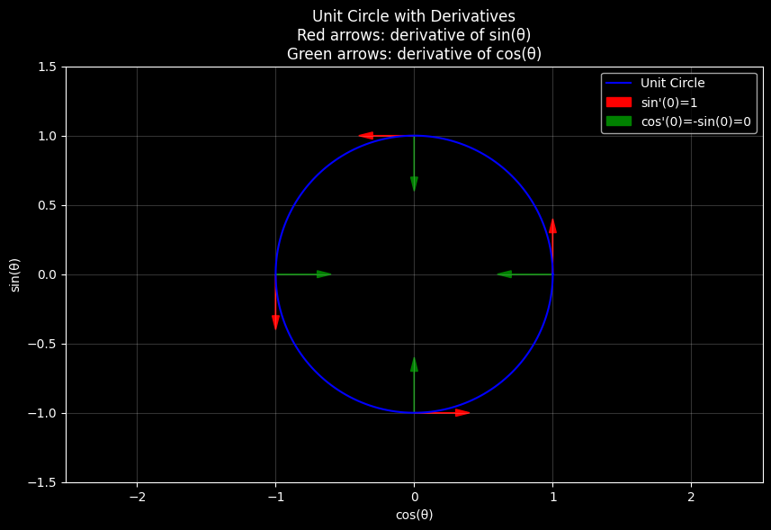 Derivatives of Sine and Cosine Functions 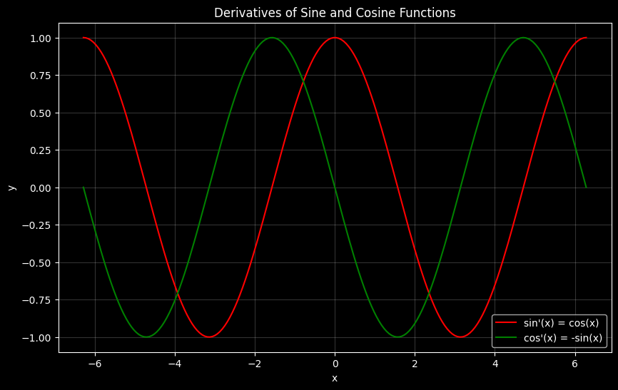 Regular Polygons with Increasing Number of Sides A regular polygon has equal sides and equal angles. Its area with $n$ sides and radius $r$ is $$A=\frac{1}{2}\,n\,r^{2}\sin\frac{2\pi}{n}$$ The radius is the straight line from the center to a corner, so the polygon splits into $n$ triangles that use that length. As the number of sides grows, the area approaches the area of the circle, $\pi r^2$. With $r=1$ that area is $\pi$. The prints below compare $\pi$, a long alternating sum that builds a number near $\pi$, and the gap between $\pi$ and the 100-sided area. ```python # Calculate area of regular polygon with n sides and radius r def regular_polygon_area(n, r): return (n * r**2 * np.sin(2*np.pi/n)) / 2 # Example: Calculate area of regular hexagon with radius 1 n = 6 r = 1 area = regular_polygon_area(n, r) print(f"Area of regular {n}-sided polygon with radius {r}: {area}") # Plot regular polygons with increasing number of sides plt.figure(figsize=(10,6)) theta = np.linspace(0, 2*np.pi, 100) r = 1 for n in [3, 4, 6, 8, 12, 32, 100]: angles = np.linspace(0, 2*np.pi, n+1) x = r * np.cos(angles) y = r * np.sin(angles) plt.plot(x, y, label=f'n={n}', linewidth=0.75) plt.axis('equal') plt.grid(True) plt.legend() plt.title('Regular Polygons with Increasing Number of Sides') plt.show() ``` 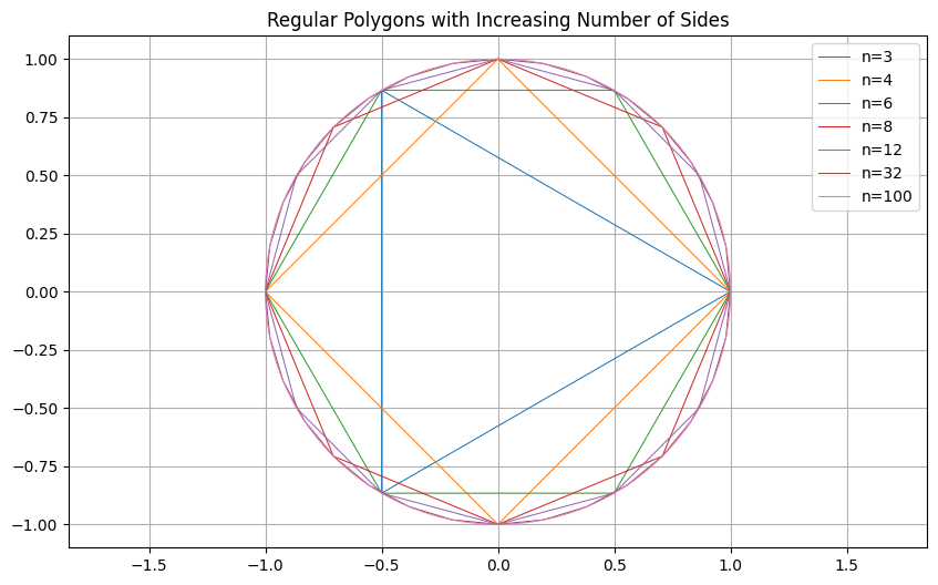 ``` 3.141592653589793 ``` ```python 4 * (1 - 1/3 + 1/5 - 1/7 + 1/9 - 1/11 + 1/13 + 1/15 - 1/17 + 1/19 - 1/21 + 1/23 - 1/25 + 1/27 - 1/29 + 1/31 - 1/33 + 1/35 - 1/37 + 1/39 - 1/41 + 1/43 - 1/45 + 1/47 - 1/49 + 1/51 - 1/53 + 1/55 - 1/57 + 1/59 - 1/61 + 1/63 - 1/65 + 1/67 - 1/69 + 1/71 - 1/73 + 1/75 - 1/77 + 1/79 - 1/81 + 1/83 - 1/85 + 1/87 - 1/89 + 1/91 - 1/93 + 1/95 - 1/97 + 1/99 - 1/101) ``` ``` 3.4062783544899182 ``` ```python np.pi - regular_polygon_area(100, 1) ``` ``` 0.0020666771241244497 ``` a growth rate that falls to 0 as x approaches 100 ```python # a growth rate that falls to 0 as x approaches 100 from math import sqrt linspace = np.linspace(0,100,1000) y = [sqrt(100-x) for x in linspace] plt.plot(np.linspace(0,100,1000),y) ``` 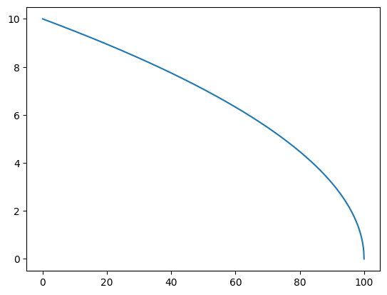 Exponential Function on Logarithmic Scale A logarithm counts how many times you multiply by a base to reach a number. On a log scale, equal steps on the axis are equal multiplications, so $e^x$, a constant near 2.718 raised to $x$, is drawn as a straight line. ```python # Create data for exponential function x = np.linspace(0, 10, 1000) y = np.exp(x) # Create figure and axis plt.figure(figsize=(10, 6)) # Plot exponential on log scale plt.semilogy(x, y, 'b-', label='y = e^x') # Customize the plot plt.grid(True, which="both", ls="-", alpha=0.2) plt.xlabel('x') plt.ylabel('y (log scale)') plt.title('Exponential Function on Logarithmic Scale') plt.legend() plt.show() ``` 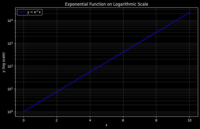 Comparison of Growth Rates $e^x$ and $2^x$ grow by multiplying by a constant at each step. $x^2$ and $x^3$ grow by raising the input to a fixed power. The exponential curves pull away from the powers. ```python # Compare e with other growth rates x = np.linspace(0, 5, 100) # Plot different growth functions plt.figure(figsize=(10, 6)) plt.plot(x, np.exp(x), 'b-', label='e^x (exponential)') plt.plot(x, x**2, 'r-', label='x^2 (quadratic)') plt.plot(x, x**3, 'g-', label='x^3 (cubic)') plt.plot(x, 2**x, 'c-', label='2^x') plt.plot(x, x, 'k-', label='x (linear)', color='lightgrey') plt.title('Comparison of Growth Rates') plt.xlabel('x') plt.ylabel('y') plt.grid(True, alpha=0.3) plt.legend() plt.show() ``` 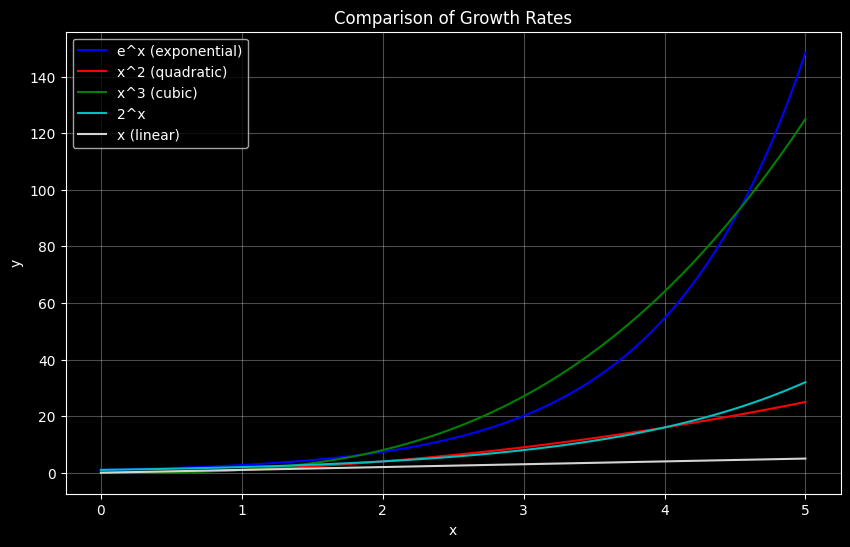 Photon Wave Function The curve drawn here is a bell-shaped envelope times a traveling ripple: $$\psi(x)=e^{-x^2/(4\sigma^2)}\,e^{i k_0 x}$$ The first factor is a Gaussian, a bell that is tall at $x=0$ and falls off on both sides. $\sigma$ sets the width. The second factor is a plane wave, a pure ripple. $k_0$ is the wave number, how many cycles sit in one unit of distance. $i$ is the imaginary unit, the number whose square is $-1$, which lets one expression carry both a cosine part and a sine part. ```python # Photon wave function (simplified quantum mechanical representation) # Using a Gaussian wave packet as an approximation x = np.linspace(-10, 10, 1000) k0 = 2 # Wave number sigma = 1.0 # Width of the wave packet # Wave function = Gaussian envelope * plane wave psi = np.exp(-(x**2)/(4*sigma**2)) * np.exp(1j*k0*x) # Plot real and imaginary parts plt.plot(x, psi.real, 'b', label='Real part') plt.plot(x, psi.imag, 'r', label='Imaginary part') plt.plot(x, abs(psi), 'g--', label='Amplitude') plt.title('Photon Wave Function') plt.xlabel('Position (arbitrary units)') plt.ylabel('Wave Function Ψ(x)') plt.grid(True, alpha=0.2) plt.legend() ``` 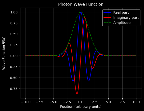 Create a 3D visualization of electromagnetic wave propagation The height of each field is a sine of distance. A sine completes one cycle over $2\pi$ radians, and a radian is the angle that marks off an arc as long as the radius. The electric field in the code is $\sin(2\pi x-\pi/2)$ and the magnetic field is $\sin(2\pi x)$. Subtracting $\pi/2$ shifts the electric field by a quarter cycle. The two fields point on perpendicular axes, and the wave travels along $x$. ```python import matplotlib.pyplot as plt from mpl_toolkits.mplot3d import Axes3D import numpy as np # Create a 3D visualization of electromagnetic wave propagation fig = plt.figure(figsize=(12, 8)) ax = fig.add_subplot(111, projection='3d') # Create data points x = np.linspace(0, 10, 100) z = np.zeros_like(x) # Electric and magnetic field components # Electric field in y direction, magnetic field in z direction # They are perpendicular to each other and to direction of propagation (x) E = np.sin(2*np.pi*x - np.pi/2) # Electric field B = np.sin(2*np.pi*x) # Magnetic field # Plot the electric field component (blue) ax.plot(x, E, z, 'b-', label='Electric field', linewidth=2) # Plot the magnetic field component (red) ax.plot(x, z, B, 'r-', label='Magnetic field', linewidth=2) # Add direction arrow for wave propagation ax.quiver(0, 0, 0, 2, 0, 0, color='green', label='Direction of propagation') # Customize the plot ax.set_xlabel('Direction of propagation (x)') ax.set_ylabel('Electric field (E)') ax.set_zlabel('Magnetic field (B)') ax.set_title('Electromagnetic Wave Propagation') # Set consistent axis limits ax.set_xlim(0, 10) ax.set_ylim(-1.5, 1.5) ax.set_zlim(-1.5, 1.5) plt.legend() plt.show() ``` 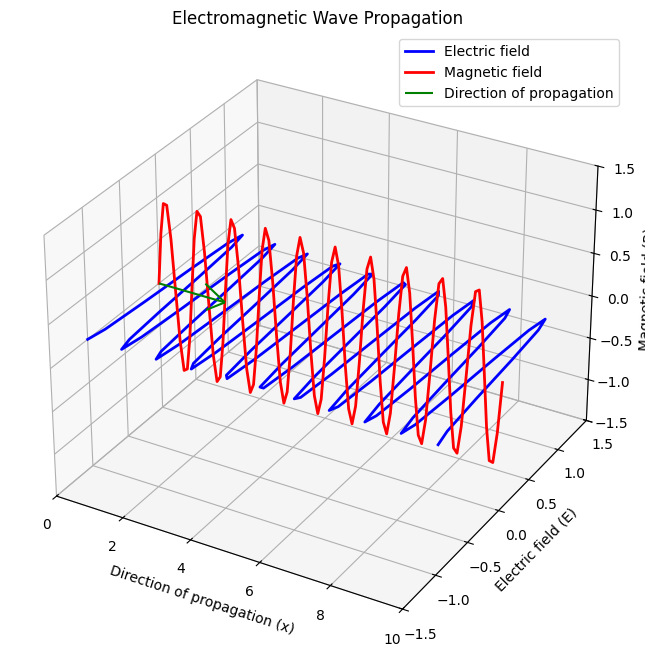 Graph of -x·sin(x) + cos(x) ```python # Plot -x·sin(x) + cos(x) x = np.linspace(-100, 100, 1000) y = -x * np.sin(x) + np.cos(x) plt.figure(figsize=(10, 6)) plt.plot(x, y, 'b-', label='-x·sin(x) + cos(x)') plt.title('Graph of -x·sin(x) + cos(x)') plt.xlabel('x') plt.ylabel('y') plt.grid(True, alpha=0.3) plt.legend() plt.show() ``` 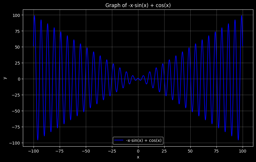 Next: [Big O](big-o.html).