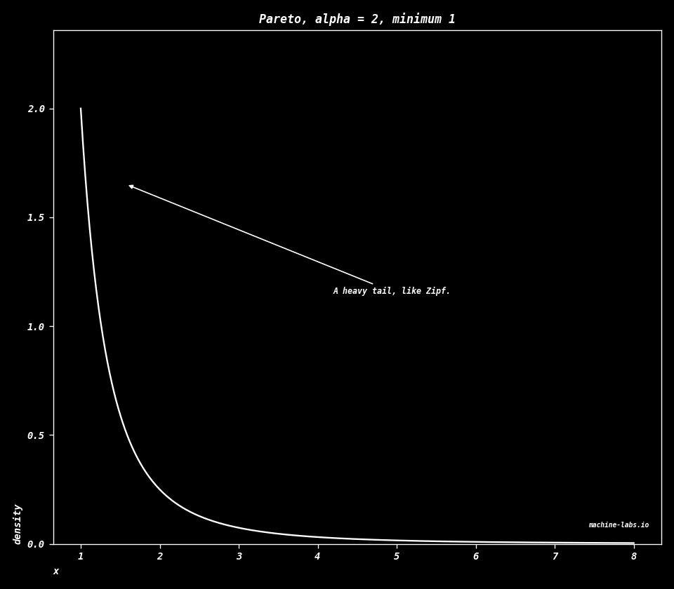
Distributions Temperature, Zipf, and the standard distribution shapes. math · distributions Study sequence: [Vectors](vectors.html) · [Matrices](matrices.html) · [Matrix applications](matrix-applications.html) · [Calculus](calculus.html) · [Big O](big-o.html) · [Geometry](geometry.html) · [Signals](signals.html) · [Neural nets](neural-nets.html) · Distributions Let's explain the temperature scaling formula for softmax probabilities The formula qi = exp(zi/T) / sum(exp(zj/T)) represents temperature-scaled softmax, where: $$q_i=\frac{\exp(z_i/T)}{\sum_j\exp(z_j/T)}$$ $\exp$ means $e$ raised to that power, and $e$ is about 2.718. $z_i$ is the raw score for class $i$, before the scores are turned into shares that add to 1. Dividing the scores by $T$ before the exponential is the temperature. A low temperature makes the biggest score take almost the whole share. A high temperature spreads the share across the classes. - qi is the output probability for class i - zi is the logit (pre-softmax activation) for class i - T is the temperature parameter - The sum in denominator is over all classes j Let's demonstrate with a simple example Calculate numerator: exp(zi/T) Calculate denominator: sum(exp(zj/T)) Calculate final probability qi Key observations: 1. Lower temperature (T<1) makes distribution more peaked/confident 2. Higher temperature (T>1) makes distribution more uniform/smooth 3. T=1 gives standard softmax without scaling ``` Numerator exp(zi/T) = 54.5982 Denominator sum(exp(zj/T)) = 62.9872 Final probability qi = 0.8668 ``` ## By hand: softmax @ alan yeh. ai by hand [https://aibyhand.substack.com/](https://aibyhand.substack.com/) ```python e = 3 e**1/30 ``` ``` 0.1 ``` The power runs before the division, so this line is $(3^1)/30=0.1$. The comment on `sm` sets $e=3$ in place of $2.71828$. [https://aibyhand.substack.com/p/w11-softmax](https://aibyhand.substack.com/p/w11-softmax) ```python def sm(x): e = 3 # 2.71828 x = np.power(e, x) return x/np.sum(x) ``` ```python sm([6,5.9]) ``` ``` array([0.52743772, 0.47256228]) ``` ```python # ex1 sm(L(M([1,1,-1],[1,-1,-1]), M([2],[1]))) ``` ``` array([[0.9], [0.1]]) ``` ```python # ex2 sm(L(M([1,1,0],[1,-1,0]), M([2],[1]))) ``` ``` array([[0.9], [0.1]]) ``` ```python # ex3 sm(L(M([1,1,1],[1,-1,1]), M([2],[1]))) ``` ``` array([[0.9], [0.1]]) ``` ```python sm(L(M([1,1,2],[1,-1,2]), M([2],[1]))) ``` ``` array([[0.9], [0.1]]) ``` ```python sm(L(M([1,1,3],[1,-1,3]), M([2],[1]))) ``` ``` array([[0.9], [0.1]]) ``` ```python sm(L(M([1,1,3],[1,-1,5]), M([2],[1]))) ``` ``` array([[0.5], [0.5]]) ``` ```python sm(L(M([1,1,2],[1,-1,4]), M([2],[1]))) ``` ``` array([[0.5], [0.5]]) ``` ```python sm(L(M([1,1,0],[1,-1,2]), M([2],[1]))) ``` ``` array([[0.5], [0.5]]) ``` ```python sm(L(M([1,1,0],[1,-1,1]), M([2],[1]))) ``` ``` array([[0.75], [0.25]]) ``` ```python sm(L(M([1,1,-1],[1,-1,-1],[1,0,-2],[0,1,1]), M([2],[1]))) ``` ``` array([[0.45], [0.05], [0.05], [0.45]]) ``` ```python sm(L(M([1,1,-1],[1,-1,3],[1,0,0],[0,1,-1]), M([2],[1]))) ``` ``` array([[0.09], [0.81], [0.09], [0.01]]) ``` ```python sm(L(M([1,1,-3],[1,-1,0],[1,0,0],[0,1,2],[1,2,-4],[2,1,-3]), M([2],[1]))) ``` ``` array([[0.02], [0.06], [0.18], [0.54], [0.02], [0.18]]) ``` temperatures 0.1, 0.5, 1.0, 2.0, 5.0 ```python # Define some example logits (pre-softmax values) logits = np.array([2.0, 1.0, 0.0, -1.0, -2.0]) # Define different temperature values to test temperatures = [0.1, 0.5, 1.0, 2.0, 5.0] # Create a figure with subplots plt.figure(figsize=(15, 5)) # Plot probability distributions for each temperature for i, temp in enumerate(temperatures, 1): plt.subplot(1, len(temperatures), i) # Apply temperature scaling and softmax scaled_logits = logits / temp probs = np.exp(scaled_logits) / np.sum(np.exp(scaled_logits)) # Create bar plot plt.bar(range(len(logits)), probs) plt.title(f'Temperature = {temp}') plt.ylim(0, 1) plt.xlabel('Class') plt.ylabel('Probability') plt.tight_layout() plt.show() ``` 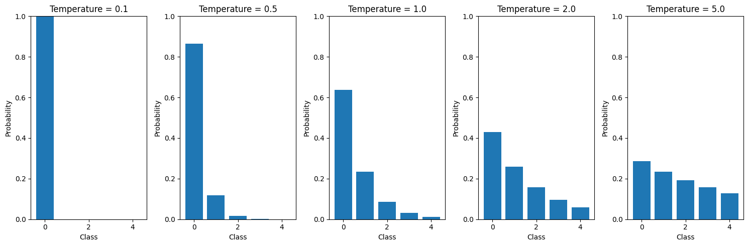 temperatures 0.1, 0.25, 0.5, 0.75, 1.0 ```python # Define some example logits (pre-softmax values) logits = np.array([2.0, 1.0, 0.0, -1.0, -2.0]) # Define different temperature values to test (between 0 and 1) temperatures = [0.1, 0.25, 0.5, 0.75, 1.0] # Create a figure with subplots plt.figure(figsize=(15, 5)) # Plot probability distributions for each temperature for i, temp in enumerate(temperatures, 1): plt.subplot(1, len(temperatures), i) # Apply temperature scaling and softmax scaled_logits = logits / temp probs = np.exp(scaled_logits) / np.sum(np.exp(scaled_logits)) # Create bar plot plt.bar(range(len(logits)), probs) plt.title(f'Temperature = {temp}') plt.ylim(0, 1) plt.xlabel('Class') plt.ylabel('Probability') plt.tight_layout() plt.show() ``` 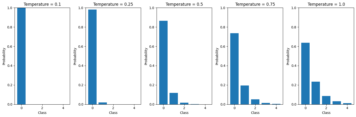 Effect of Temperature on Token Selection Probabilities (Approaching T=0) ```python # Create a concrete example of transformer token selection with temperature=0 import numpy as np import matplotlib.pyplot as plt # Sample logits for next token prediction (pre-softmax scores) # Let's simulate scores for 5 candidate tokens tokens = ['cat', 'dog', 'bird', 'fish', 'rabbit'] logits = np.array([2.5, 1.8, 0.9, 0.4, 0.2]) # Create figure with 5 subplots showing probability distribution at different temperatures fig, axes = plt.subplots(1, 5, figsize=(15, 5)) temperatures = [1.0, 0.5, 0.2, 0.1, 0.01] for i, temp in enumerate(temperatures): # Apply temperature scaling and softmax scaled_logits = logits / temp probs = np.exp(scaled_logits) / np.sum(np.exp(scaled_logits)) # Plot probabilities as bars axes[i].bar(tokens, probs) axes[i].set_title(f'T = {temp}') axes[i].set_ylim(0, 1) axes[i].tick_params(axis='x', rotation=45) # Annotate probabilities for j, prob in enumerate(probs): axes[i].text(j, prob + 0.02, f'{prob:.2f}', ha='center') plt.suptitle('Effect of Temperature on Token Selection Probabilities\n(Approaching T=0)') plt.tight_layout() plt.show() # Print analysis of what happens as T approaches 0 print("\nAs temperature approaches 0:") print("- The highest scoring token ('cat') gets increasingly dominant") print("- Other token probabilities approach 0") print("- At T=0.01, selection becomes nearly deterministic") print(f"- Probability of 'cat' at T=0.01: {probs[0]:.4f}") ``` 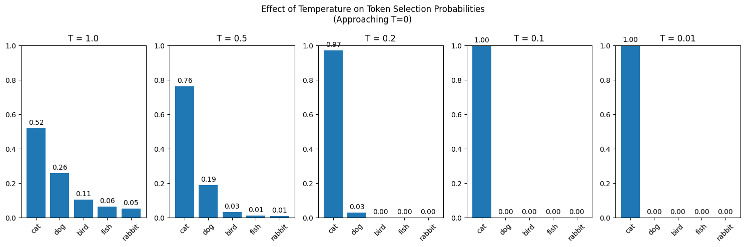 Zipf Zipf's law says the frequency of the item at rank $k$ is proportional to $1/k$: $$f(k)\propto\frac{1}{k}$$ Proportional means one quantity is a constant times the other. The most common item is about twice the second and about three times the third. On a log-log plot both axes are logarithmic, equal steps meaning equal multiplications, and $1/k$ is a straight line. The token plots below are this same shape, with some wobble added. A token is one piece of text being scored, often a word or a piece of a word. A distribution is a list of shares across outcomes. Temperature and Zipf are two readings of how uneven that list is. ```python # Example of Zipf's Law for word frequencies import numpy as np import matplotlib.pyplot as plt # Generate ranks from 1 to 1000 ranks = np.arange(1, 1001) # Calculate frequencies using Zipf's Law: frequency ∝ 1/rank frequencies = 1/ranks # Create the plot plt.figure(figsize=(10, 6)) plt.loglog(ranks, frequencies, 'b-', label="Zipf's Law") plt.grid(True) plt.title("Zipf's Law: Word Frequency vs Rank") plt.xlabel('Word Rank (log scale)') plt.ylabel('Relative Frequency (log scale)') plt.legend() # Add text annotation explaining Zipf's Law plt.text(0.95, 0.95, "Zipf's Law states that the frequency of any word\n" + "is inversely proportional to its rank in the\n" + "frequency table", transform=plt.gca().transAxes, verticalalignment='top', horizontalalignment='right', bbox=dict(facecolor='white', alpha=0.8)) plt.tight_layout() plt.show() ``` 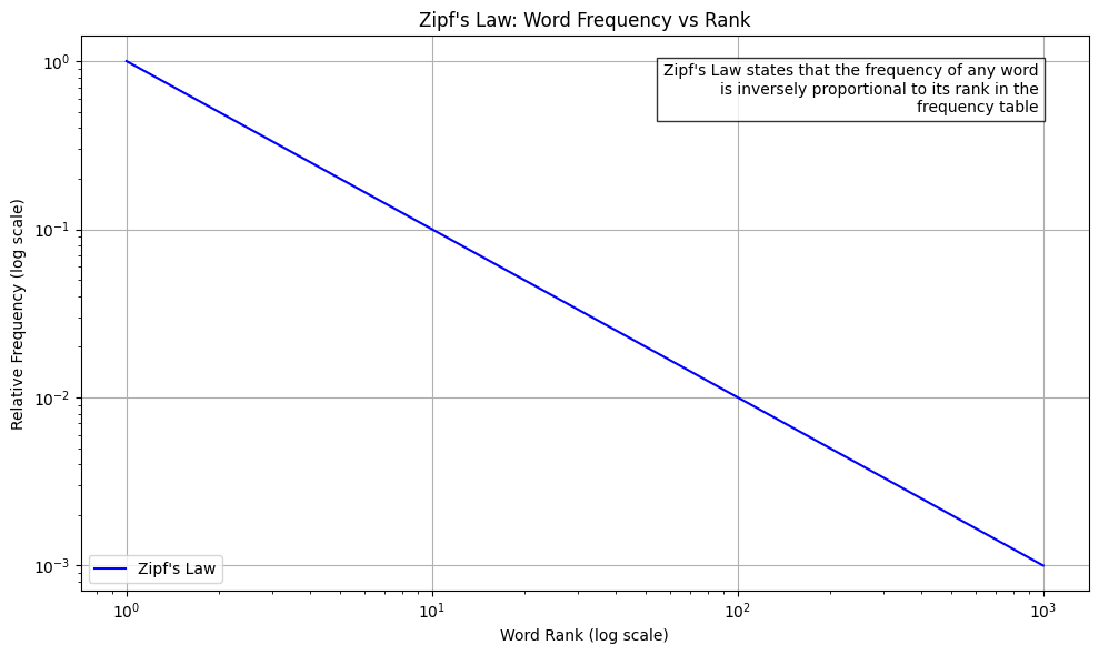 Frequency Distribution of Subword Tokens ```python # Example of subword tokenization frequency distribution import numpy as np import matplotlib.pyplot as plt # Sample text for tokenization (you may want to use your actual tokenized data) text = "The quick brown fox jumps over the lazy dog. This is a sample text to demonstrate subword tokenization." # Simulate subword token frequencies (replace this with actual tokenizer output) # This is a simplified example - actual subword distributions may vary n_tokens = 100 # Generate frequencies that follow roughly Zipfian distribution but with some variation frequencies = np.random.pareto(1, n_tokens) frequencies = frequencies / frequencies.sum() # Normalize # Sort frequencies in descending order frequencies = np.sort(frequencies)[::-1] ranks = np.arange(1, len(frequencies) + 1) # Create the plot plt.figure(figsize=(10, 6)) plt.loglog(ranks, frequencies, 'r-', label='Subword tokens') plt.grid(True) plt.title('Frequency Distribution of Subword Tokens') plt.xlabel('Token Rank (log scale)') plt.ylabel('Relative Frequency (log scale)') plt.legend() # Add text annotation plt.text(0.95, 0.95, "Subword tokenization often results in a\n" + "distribution similar to Zipf's Law, but with\n" + "some characteristic differences due to the\n" + "nature of subword splitting", transform=plt.gca().transAxes, verticalalignment='top', horizontalalignment='right', bbox=dict(facecolor='white', alpha=0.8)) plt.tight_layout() plt.show() ``` 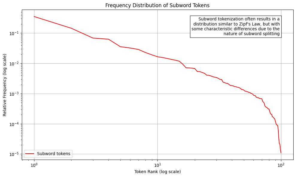 Token Probability Distribution in Transformer Output ```python # Analyzing token distribution in response to natural language prompts import numpy as np import matplotlib.pyplot as plt # Simulate token probabilities from a transformer's output distribution # This represents the probability distribution over the vocabulary after processing a prompt n_tokens = 1000 # Generate a more peaked distribution typical of transformer outputs # Using modified softmax-like distribution x = np.linspace(0, 10, n_tokens) logits = np.exp(-x/2) + 0.1*np.random.random(n_tokens) probabilities = logits / logits.sum() # Sort probabilities in descending order probabilities = np.sort(probabilities)[::-1] ranks = np.arange(1, len(probabilities) + 1) # Create the plot plt.figure(figsize=(10, 6)) plt.loglog(ranks, probabilities, 'b-', label='Token probabilities') plt.grid(True) plt.title('Token Probability Distribution in Transformer Output') plt.xlabel('Token Rank (log scale)') plt.ylabel('Probability (log scale)') plt.legend() # Add text annotation explaining the distribution plt.text(0.95, 0.95, "Transformer output distributions tend to be:\n" + "• More peaked than Zipfian\n" + "• Concentrated on contextually relevant tokens\n" + "• Influenced by attention patterns\n" + "• Temperature-dependent in sampling", transform=plt.gca().transAxes, verticalalignment='top', horizontalalignment='right', bbox=dict(facecolor='white', alpha=0.8)) plt.tight_layout() plt.show() ``` 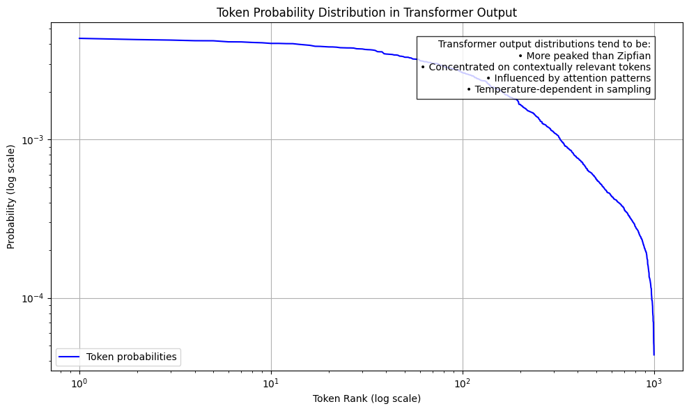 Token Probability Distribution with Temperature=0 ```python # Analyzing token distribution with temperature=0 (deterministic/greedy sampling) import numpy as np import matplotlib.pyplot as plt # Simulate token probabilities with temperature=0 # This will create a much more peaked distribution where probability mass concentrates on top tokens n_tokens = 1000 x = np.linspace(0, 10, n_tokens) logits = np.exp(-x/2) + 0.1*np.random.random(n_tokens) # Apply temperature=0 effect (approaches one-hot) # We'll simulate this by heavily concentrating probability mass on top tokens temperature = 0.01 # Very close to 0 (avoiding division by 0) logits = logits/temperature probabilities = np.exp(logits) / np.sum(np.exp(logits)) # Sort probabilities in descending order probabilities = np.sort(probabilities)[::-1] ranks = np.arange(1, len(probabilities) + 1) # Create the plot plt.figure(figsize=(10, 6)) plt.loglog(ranks, probabilities, 'r-', label='Token probabilities (T=0)') plt.grid(True) plt.title('Token Probability Distribution with Temperature=0') plt.xlabel('Token Rank (log scale)') plt.ylabel('Probability (log scale)') plt.legend() # Add text annotation explaining the effect of temperature=0 plt.text(0.95, 0.95, "Temperature=0 characteristics:\n" + "• Approaches deterministic selection\n" + "• Highest probability token dominates\n" + "• Very steep probability drop-off\n" + "• Used for maximum likelihood sampling", transform=plt.gca().transAxes, verticalalignment='top', horizontalalignment='right', bbox=dict(facecolor='white', alpha=0.8)) plt.tight_layout() plt.show() ``` 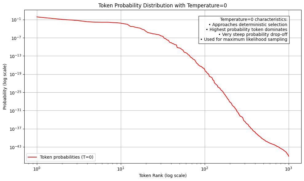 # Distribution shapes A distribution is a rule that hands out shares of certainty across outcomes. A discrete outcome is a separate value, such as a count or the face of a die. Its probability mass function, the pmf, is the probability of that exact value. A continuous outcome can fall anywhere along a stretch of the number line. Its probability density function, the pdf, is the height of a curve, and the probability is the area under the curve between two points. A parameter is a fixed number chosen before the curve is drawn. It sets the shape. The charts use the black field and the white mark from [Big O](big-o.html). `dplot` is that style. Each block below builds one distribution and draws it. The equation above the block is the curve the code evaluates. ## The chart ```python import numpy as np import matplotlib.pyplot as plt from scipy import stats def dplot(x, y, title, xlab, ylab, kind="line", note=None, filename=None, note_at=None, arrow_at=None): fig = plt.figure(facecolor="#000000", edgecolor="#000000", figsize=(8, 7), layout="tight") ax = plt.axes(facecolor="#000000") ax.tick_params(colors="white") plt.xticks(fontfamily="monospace", fontsize="small", fontstyle="italic", fontweight="semibold") plt.yticks(fontfamily="monospace", fontsize="small", fontstyle="italic", fontweight="semibold") plt.title(title, fontfamily="monospace", fontsize="medium", fontstyle="italic", fontweight="semibold", color="#ffffff") plt.xlabel(xlab, loc="left", fontfamily="monospace", fontsize="small", fontstyle="italic", fontweight="semibold", color="#ffffff") plt.ylabel(ylab, loc="bottom", fontfamily="monospace", fontsize="small", fontstyle="italic", fontweight="semibold", color="#ffffff") for spine in ax.spines.values(): spine.set_color("#ffffff") y = np.asarray(y, dtype=float) x = np.asarray(x, dtype=float) if kind == "stem": pad = 0.6 plt.xlim(float(x.min()) - pad, float(x.max()) + pad) plt.vlines(x, 0, y, color="#ffffff", linewidth=1) plt.plot(x, y, linestyle="none", marker="o", color="#ffffff", markersize=4.5) plt.ylim(0, float(y.max()) * 1.28) else: plt.plot(x, y, color="#ffffff", linewidth=1.4) plt.ylim(0, float(y.max()) * 1.18) if note: if note_at is None or arrow_at is None: xi = int(np.argmax(y)) xlim = ax.get_xlim() ylim = ax.get_ylim() px = (x[xi] - xlim[0]) / (xlim[1] - xlim[0]) py = (y[xi] - ylim[0]) / (ylim[1] - ylim[0]) px = float(np.clip(px, 0.08, 0.92)) py = float(np.clip(py * 0.92, 0.12, 0.78)) if note_at is None: note_at = (0.08, 0.86) if px > 0.45 else (0.46, 0.86) if arrow_at is None: arrow_at = (px, py) ax.annotate( note, xy=arrow_at, xytext=note_at, xycoords="axes fraction", textcoords="axes fraction", arrowprops={"arrowstyle": "-|>", "color": "#ffffff"}, color="#ffffff", fontfamily="monospace", fontsize="x-small", fontstyle="italic", fontweight="semibold", ha="left", va="top", ) ax.text( 0.98, 0.03, "machine-labs.io", transform=ax.transAxes, ha="right", va="bottom", color="#ffffff", fontfamily="monospace", fontsize="xx-small", fontstyle="italic", fontweight="semibold", ) if filename is not None: fig.savefig(filename, facecolor="#000000", edgecolor="#000000", dpi=120) plt.close(fig) ``` ## Discrete uniform A fair die. Each face is a separate outcome, and each face gets the same share. $n$ is how many faces there are. Here $n=6$. $$P(X=k)=\frac{1}{n},\quad k=1,2,\ldots,n$$ ```python x = np.arange(1, 7) y = stats.randint.pmf(x, 1, 7) dplot( x, y, title="Discrete uniform, 1 to 6", xlab="face", ylab="probability", kind="stem", note="Every face, the same share.", filename="d-uniform-discrete.png", note_at=(0.18, 0.55), arrow_at=(0.55, 0.78), ) ``` 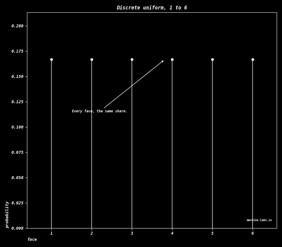 ## Bernoulli One trial with two outcomes. Call outcome 1 a success. $p$ is the probability of that success. Outcome 0 gets the rest of the share, $1-p$. $$P(X=1)=p,\qquad P(X=0)=1-p$$ ```python p = 0.3 x = np.array([0, 1]) y = stats.bernoulli.pmf(x, p) dplot( x, y, title="Bernoulli, p = 0.3", xlab="outcome", ylab="probability", kind="stem", note="One yes-or-no trial.", filename="d-bernoulli.png", note_at=(0.38, 0.58), arrow_at=(0.73, 0.36), ) ``` 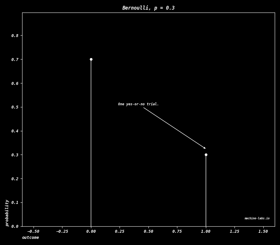 ## Binomial Repeat an independent Bernoulli trial $n$ times and count the successes. Independent means one trial leaves the next trial's $p$ unchanged. $\binom{n}{k}$ is the number of ways to choose which $k$ of the $n$ trials are the successes. $$P(X=k)=\binom{n}{k}p^{k}(1-p)^{n-k},\quad k=0,1,\ldots,n$$ ```python n, p = 20, 0.4 x = np.arange(0, n + 1) y = stats.binom.pmf(x, n, p) dplot( x, y, title="Binomial, n = 20, p = 0.4", xlab="successes k", ylab="probability", kind="stem", note="Successes in n trials.", filename="d-binomial.png", ) ``` 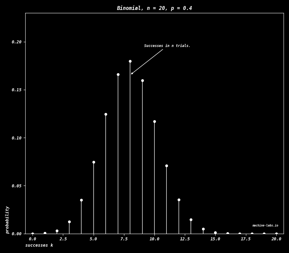 ## Poisson The count of events in a fixed window, when the events are rare and each one arrives on its own. $\lambda$ is the average count, the balance point of the shares. $k!$ is the factorial, the product $1\times 2\times\cdots\times k$. $e$ is about 2.718. The chart uses $\lambda=4$. $$P(X=k)=\frac{\lambda^{k} e^{-\lambda}}{k!},\quad k=0,1,2,\ldots$$ ```python lam = 4 x = np.arange(0, 16) y = stats.poisson.pmf(x, lam) dplot( x, y, title="Poisson, lambda = 4", xlab="count k", ylab="probability", kind="stem", note="Count of rare events.", filename="d-poisson.png", ) ``` 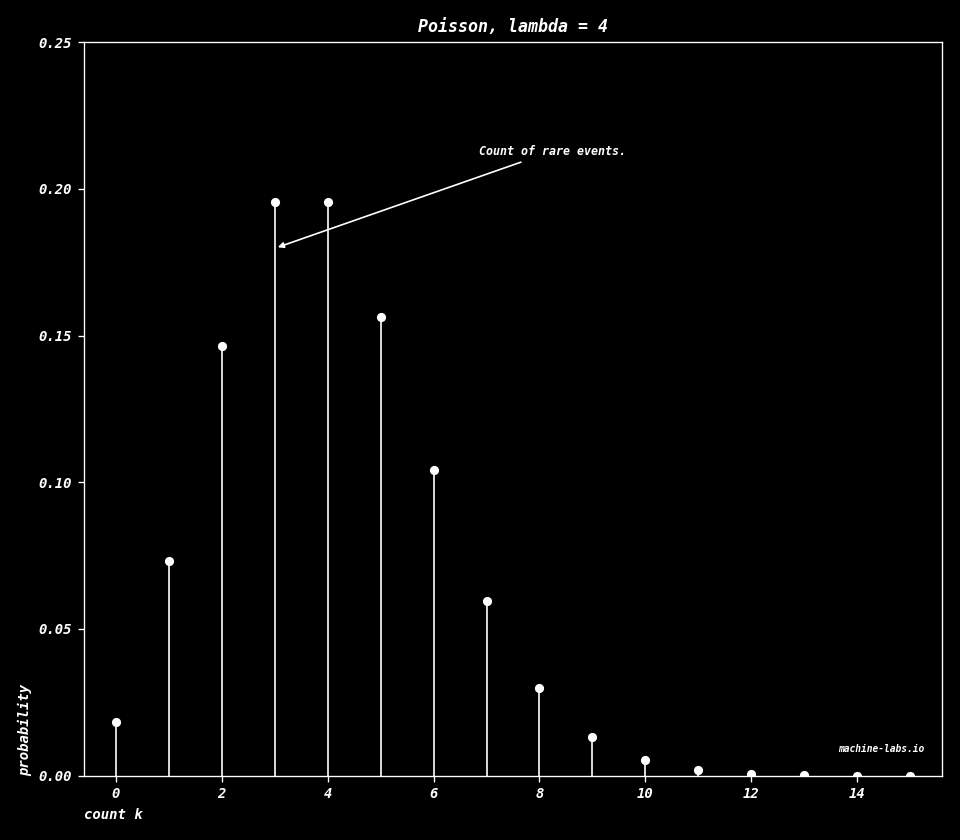 ## Geometric Keep running independent Bernoulli trials until the first success. $k$ is the trial number of that success. The first trial is the most likely place for it, and each later trial is scaled by another factor of $1-p$. $$P(X=k)=(1-p)^{k-1}p,\quad k=1,2,3,\ldots$$ ```python p = 0.3 x = np.arange(1, 16) y = stats.geom.pmf(x, p) dplot( x, y, title="Geometric, p = 0.3", xlab="trial k of first success", ylab="probability", kind="stem", note="Trials until first success.", filename="d-geometric.png", note_at=(0.34, 0.62), arrow_at=(0.10, 0.74), ) ```  ## Continuous uniform Every stretch of equal length inside an interval gets the same probability. The density is the height of the curve, and the probability is the area under it. Here the interval runs from $a=0$ to $b=1$, so the height is $1$, and the rectangle has area $1$. Outside the interval the density is $0$. $$f(x)=\frac{1}{b-a},\quad a\le x\le b$$ ```python a, b = 0.0, 1.0 x = np.linspace(a, b, 400) y = stats.uniform.pdf(x, loc=a, scale=b - a) dplot( x, y, title="Continuous uniform, 0 to 1", xlab="x", ylab="density", note="Flat on an interval.", filename="d-uniform.png", note_at=(0.16, 0.45), arrow_at=(0.55, 0.78), ) ```  ## Normal The bell. $\mu$ is the mean, the balance point. $\sigma$ is the standard deviation, the usual width. About two thirds of the draws fall within one standard deviation of the mean. This chart is the standard normal, $\mu=0$ and $\sigma=1$. The same bell is the Gaussian kernel in [Matrix applications](matrix-applications.html#image-feature-detection-with-convolution). $$f(x)=\frac{1}{\sigma\sqrt{2\pi}}\exp\left(-\frac{(x-\mu)^{2}}{2\sigma^{2}}\right)$$ ```python mu, sigma = 0.0, 1.0 x = np.linspace(-4, 4, 500) y = stats.norm.pdf(x, loc=mu, scale=sigma) dplot( x, y, title="Normal, mean 0, width 1", xlab="x", ylab="density", note="The bell.", filename="d-normal.png", ) ```  ## Exponential A waiting time. The rate $\lambda$ is how many events you expect per unit of time. In every equal slice of time, the chance of still waiting falls by the same fraction, at every age of the wait. The chart uses $\lambda=1$, so the height at $0$ is $1$. $$f(x)=\lambda e^{-\lambda x},\quad x\ge 0$$ ```python lam = 1.0 x = np.linspace(0, 8, 500) y = stats.expon.pdf(x, scale=1 / lam) dplot( x, y, title="Exponential, rate 1", xlab="x", ylab="density", note="A waiting time.", filename="d-exponential.png", note_at=(0.48, 0.55), arrow_at=(0.18, 0.62), ) ```  ## Gamma Add $k$ independent exponential waits that share a scale $\theta$. The shape $k$ is that count, and the scale stretches the time. $\Gamma(k)$, the gamma function, extends the factorial past the whole numbers. For a whole number, $\Gamma(k)=(k-1)!$. The chart uses $k=3$ and $\theta=1$. $$f(x)=\frac{1}{\Gamma(k)\,\theta^{k}}x^{k-1}e^{-x/\theta},\quad x\ge 0$$ ```python k, theta = 3.0, 1.0 x = np.linspace(0, 12, 500) y = stats.gamma.pdf(x, a=k, scale=theta) dplot( x, y, title="Gamma, shape 3, scale 1", xlab="x", ylab="density", note="Sum of exponential waits.", filename="d-gamma.png", ) ``` 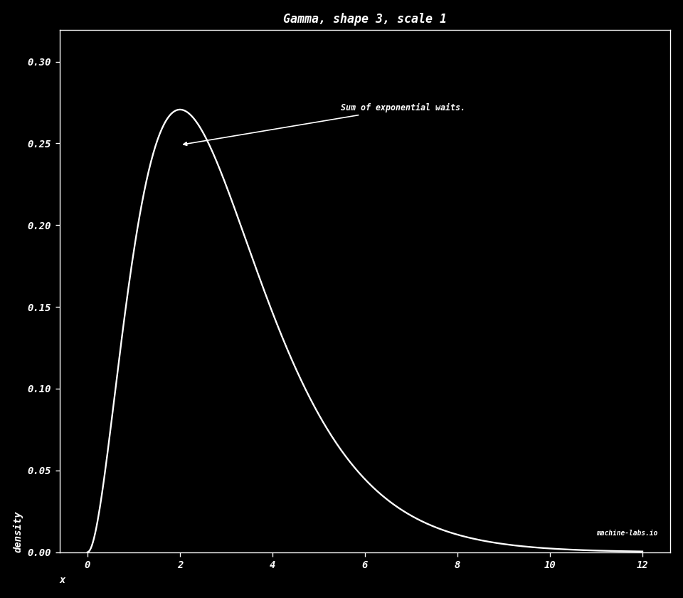 ## Chi-square Take $\nu$ independent standard normal draws and add their squares. A standard normal has mean $0$ and width $1$. $\nu$ is the degrees of freedom, that count of squares. Chi-square is a gamma with shape $\nu/2$ and scale $2$. The chart uses $\nu=4$. $$f(x)=\frac{1}{2^{\nu/2}\Gamma(\nu/2)}x^{\nu/2-1}e^{-x/2},\quad x\ge 0$$ ```python nu = 4 x = np.linspace(0.05, 16, 500) y = stats.chi2.pdf(x, nu) dplot( x, y, title="Chi-square, nu = 4", xlab="x", ylab="density", note="Sum of squared normals.", filename="d-chi-square.png", ) ``` 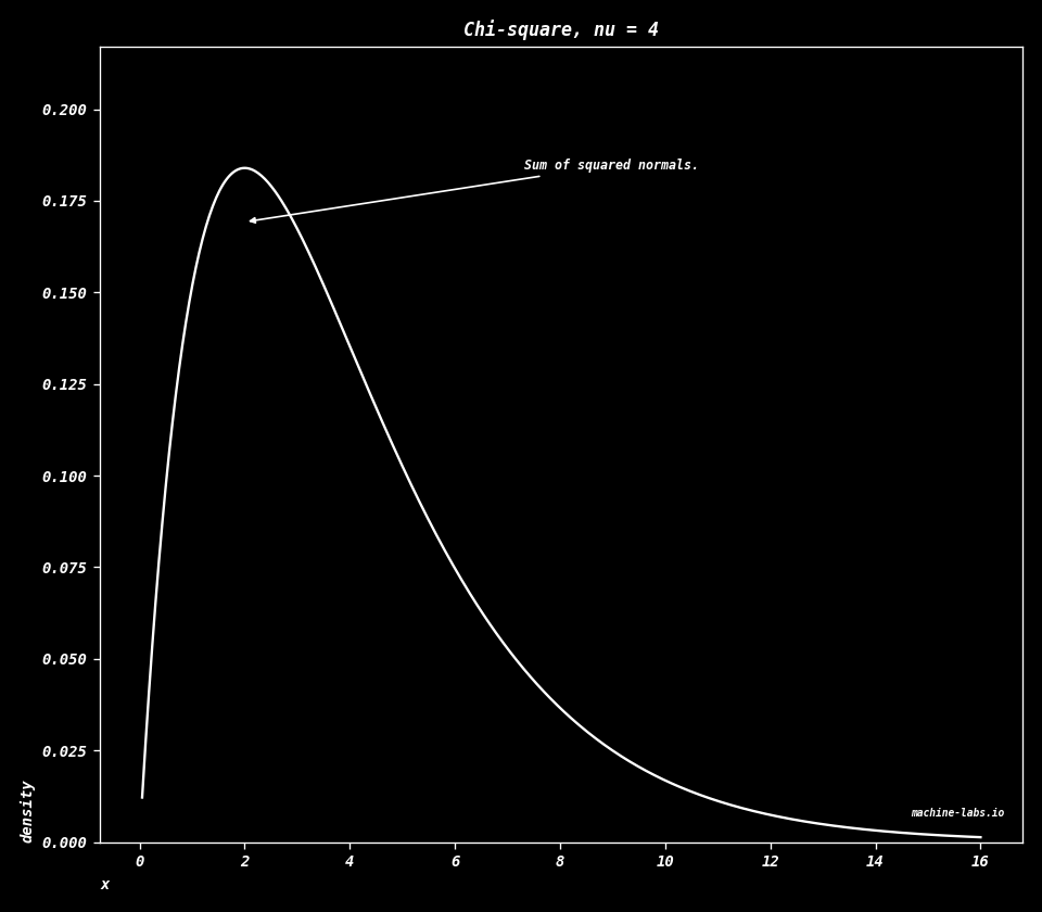 ## Beta A random share, a number from $0$ to $1$. $\alpha$ pulls the share upward. $\beta$ pulls it downward. With $\alpha=2$ and $\beta=5$ the pile sits toward the small shares. $$f(x)=\frac{\Gamma(\alpha+\beta)}{\Gamma(\alpha)\Gamma(\beta)}x^{\alpha-1}(1-x)^{\beta-1},\quad 0\le x\le 1$$ ```python alpha, beta = 2.0, 5.0 x = np.linspace(0.001, 0.999, 500) y = stats.beta.pdf(x, alpha, beta) dplot( x, y, title="Beta, alpha = 2, beta = 5", xlab="share x", ylab="density", note="A share between 0 and 1.", filename="d-beta.png", note_at=(0.48, 0.55), arrow_at=(0.28, 0.7), ) ``` 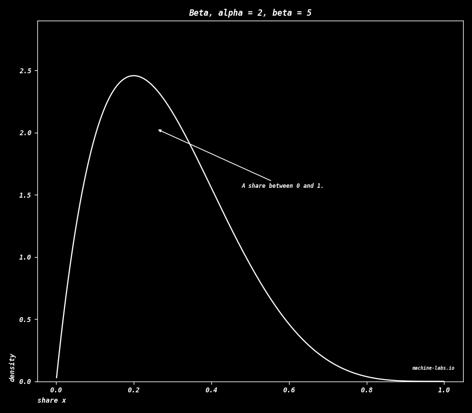 ## Student's t Start from a normal draw and divide by a width that itself comes from a chi-square with $\nu$ degrees of freedom. A tail is the far end of the curve. Small $\nu$ leaves heavy tails, more chance far from the center than the normal bell has. As $\nu$ grows, this curve settles onto the normal. The chart uses $\nu=3$. $$f(x)=\frac{\Gamma\left(\frac{\nu+1}{2}\right)}{\sqrt{\nu\pi}\,\Gamma\left(\frac{\nu}{2}\right)}\left(1+\frac{x^{2}}{\nu}\right)^{-\frac{\nu+1}{2}}$$ ```python nu = 3 x = np.linspace(-6, 6, 500) y = stats.t.pdf(x, nu) dplot( x, y, title="Student t, nu = 3", xlab="x", ylab="density", note="Heavier tails than the bell.", filename="d-student-t.png", ) ``` 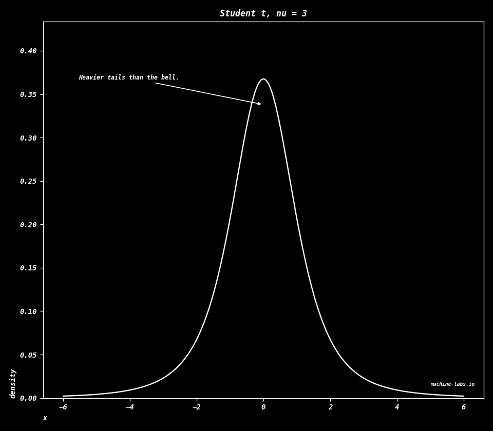 ## Lognormal Take a normal number with mean $\mu$ and width $\sigma$, and raise $e$ to that power. The logarithm of the result, how many times you multiply by $e$ to reach it, is normal. The values are positive. They pile up on the small ones and leave a long tail toward the large ones. In the code, `scale` is $e^{\mu}$ and `s` is $\sigma$. $$f(x)=\frac{1}{x\sigma\sqrt{2\pi}}\exp\left(-\frac{(\ln x-\mu)^{2}}{2\sigma^{2}}\right),\quad x>0$$ ```python mu, sigma = 0.0, 0.5 x = np.linspace(0.02, 4, 500) y = stats.lognorm.pdf(x, s=sigma, scale=np.exp(mu)) dplot( x, y, title="Lognormal, mu = 0, sigma = 0.5", xlab="x", ylab="density", note="Log of the value is normal.", filename="d-lognormal.png", note_at=(0.46, 0.55), arrow_at=(0.22, 0.7), ) ``` 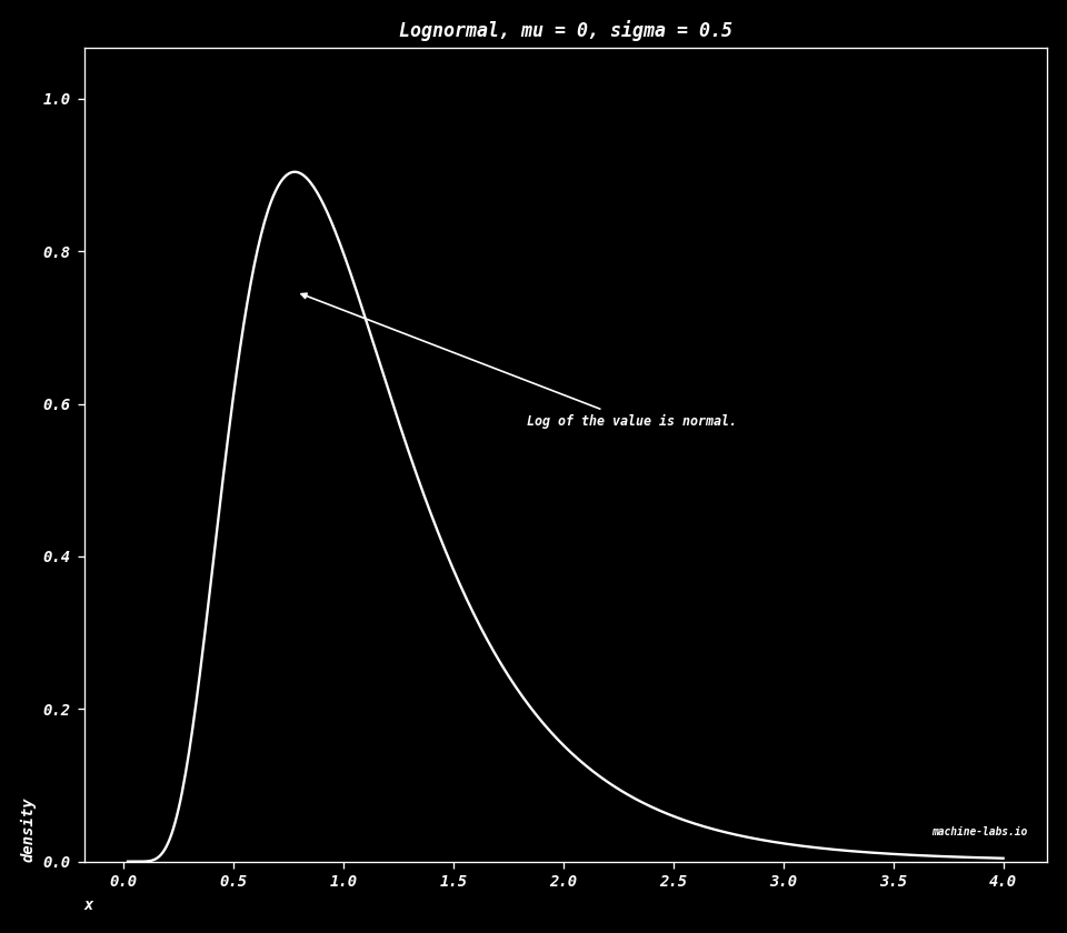 ## Weibull A model of time until something breaks. The shape $k$ says how age changes the chance of breaking in the next moment. $k=1$ is the exponential, and that chance stays the same at every age. $k$ above $1$ means an older item is more likely to break in the next moment. $\lambda$ is the scale, a typical time. The chart uses $k=1.5$ and $\lambda=1$. $$f(x)=\frac{k}{\lambda}\left(\frac{x}{\lambda}\right)^{k-1}\exp\left(-\left(\frac{x}{\lambda}\right)^{k}\right),\quad x\ge 0$$ ```python k, lam = 1.5, 1.0 x = np.linspace(0.001, 4, 500) y = stats.weibull_min.pdf(x, c=k, scale=lam) dplot( x, y, title="Weibull, shape 1.5, scale 1", xlab="x", ylab="density", note="Time until a break.", filename="d-weibull.png", ) ``` 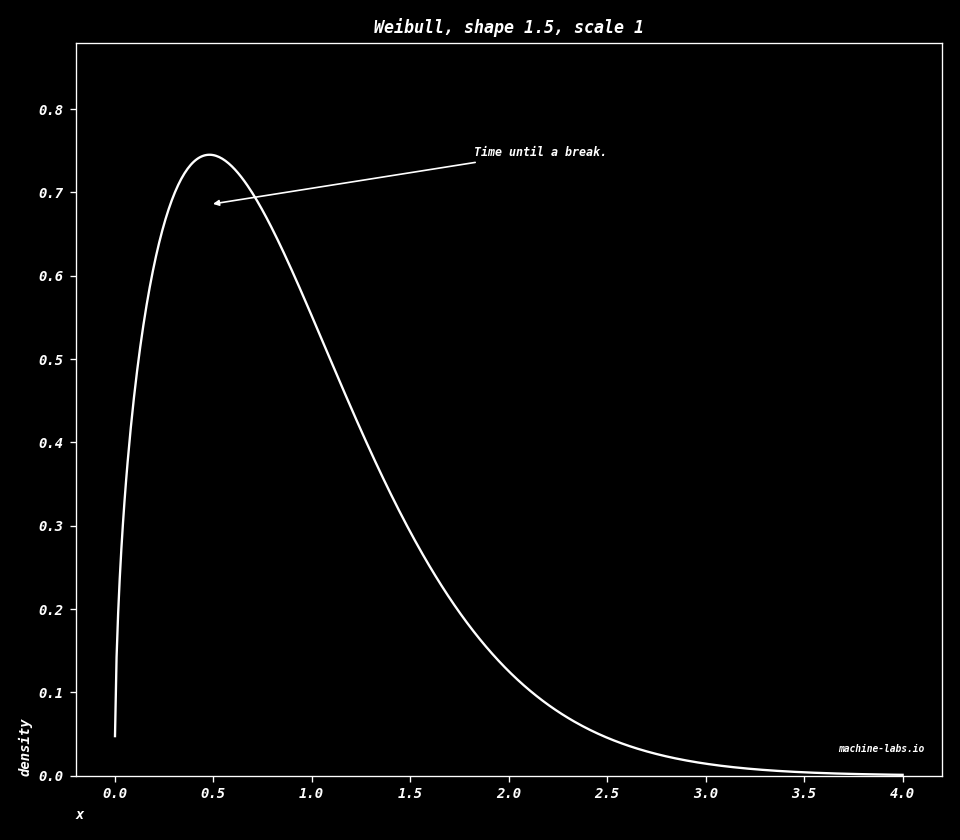 ## Laplace A sharp peak at the center $\mu$, with an exponential tail on each side. The scale $b$ sets how fast those tails fall. $$f(x)=\frac{1}{2b}\exp\left(-\frac{|x-\mu|}{b}\right)$$ ```python mu, b = 0.0, 1.0 x = np.linspace(-6, 6, 500) y = stats.laplace.pdf(x, loc=mu, scale=b) dplot( x, y, title="Laplace, center 0, scale 1", xlab="x", ylab="density", note="A sharp peak, two tails.", filename="d-laplace.png", ) ``` 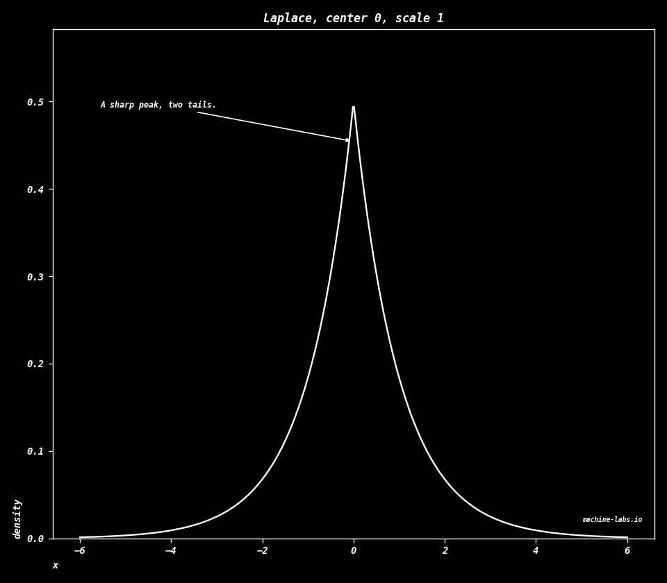 ## Logistic The running share up to $x$ is the probability of landing at $x$ or anywhere below it. With center $0$ and scale $1$, that running share is the sigmoid in [Calculus](calculus.html). This chart is the slope of that sigmoid. $$f(x)=\frac{e^{-(x-\mu)/s}}{s\left(1+e^{-(x-\mu)/s}\right)^{2}}$$ ```python mu, s = 0.0, 1.0 x = np.linspace(-8, 8, 500) y = stats.logistic.pdf(x, loc=mu, scale=s) dplot( x, y, title="Logistic, center 0, scale 1", xlab="x", ylab="density", note="Slope of the sigmoid.", filename="d-logistic.png", ) ``` 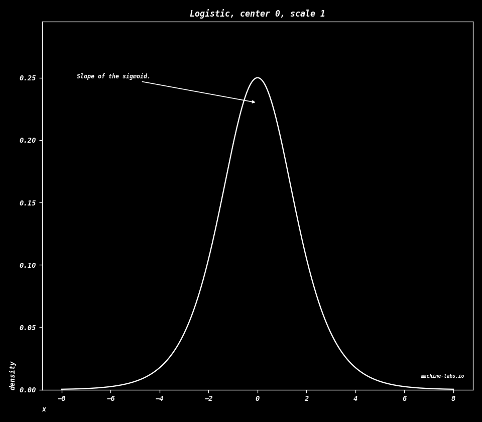 ## Cauchy A bell whose tails fall slowly. A tail is the far end of the curve. Rare huge values keep arriving, so the average of the draws keeps moving. The scale $\gamma$ sets the width. The height at the center is $1/(\pi\gamma)$. $$f(x)=\frac{1}{\pi\gamma\left(1+\left(\frac{x-x_{0}}{\gamma}\right)^{2}\right)}$$ ```python x0, gamma = 0.0, 1.0 x = np.linspace(-8, 8, 800) y = stats.cauchy.pdf(x, loc=x0, scale=gamma) dplot( x, y, title="Cauchy, center 0, scale 1", xlab="x", ylab="density", note="Tails too heavy for a mean.", filename="d-cauchy.png", ) ```  ## Pareto Values of at least $x_m$. The density falls as a power of $x$, and $\alpha$ sets how fast. A small $\alpha$ leaves a heavy tail, a lot of the share sitting on very large values. The Zipf charts above are that same fall, written for ranks instead of sizes. The chart uses $\alpha=2$ and $x_m=1$. $$f(x)=\frac{\alpha x_{m}^{\alpha}}{x^{\alpha+1}},\quad x\ge x_{m}$$ ```python alpha, xm = 2.0, 1.0 x = np.linspace(xm, 8, 500) y = stats.pareto.pdf(x, b=alpha, scale=xm) dplot( x, y, title="Pareto, alpha = 2, minimum 1", xlab="x", ylab="density", note="A heavy tail, like Zipf.", filename="d-pareto.png", note_at=(0.46, 0.5), arrow_at=(0.12, 0.7), ) ```