Matrices Bold letters, sized as rows by columns. Math counts from 1, Python from 0. math · matrices Study sequence: [Vectors](vectors.html) · Matrices · [Matrix applications](matrix-applications.html) · [Calculus](calculus.html) · [Big O](big-o.html) · [Geometry](geometry.html) · [Signals](signals.html) · [Neural nets](neural-nets.html) · [Distributions](distributions.html) # Matrices $$ \begin{bmatrix} 1 & 2\\ \pi & 4\\ 6 & 7 \end{bmatrix} \quad \begin{bmatrix} -6 & 1/3\\ e^{4.3} & -1.4\\ 6/5 & 0 \end{bmatrix} $$ Denoted with bold letters like matrix $\mathbf{A}$. Size indicated with (row, column). For instance, a 3 x 5 matrix has three rows and five columns: $$ \mathbf{M} = \begin{bmatrix} 1 & 3 & 5 & 7 & 9\\ 0 & 2 & 4 & 6 & 8\\ 1 & 4 & 7 & 8 & 9 \end{bmatrix} $$ Reference elements by indexing row and column, so the 3rd row and 4th column of matrix $\mathbf{M}$ would be $m_{3,4}=8$. **Note**, math is 1-based indexing, while Python is 0-based indexing. Matrix slicing or mrows = 5 ncols = 10 M = np.random.randn(mrows, ncols) ``` Original matrix: [[ 0 1 2 3 4 5 6 7 8 9] [10 11 12 13 14 15 16 17 18 19] [20 21 22 23 24 25 26 27 28 29] [30 31 32 33 34 35 36 37 38 39] [40 41 42 43 44 45 46 47 48 49]] Submatrix: [[10 11 12 13 14] [20 21 22 23 24] [30 31 32 33 34]] ``` square matrix ```python m = 5 n = 5 print('square matrix') print(np.random.randn(m, n)) plt.close() plt.matshow(np.random.randn(m, n)) plt.show() ``` 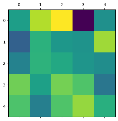 rectangular matrix ```python m = 10 n = 5 print('rectangular matrix') print(np.random.randn(m, n)) plt.close() plt.matshow(np.random.randn(m, n)) plt.show() ``` 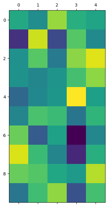 diagonal matrix ```python print('diagonal matrix') print(np.diag(range(10))) plt.close() plt.matshow(np.diag(range(10))) plt.show() ``` 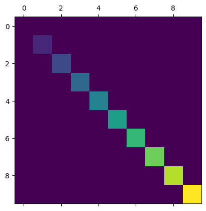 upper triangular matrix ```python print('upper triangular matrix') print(np.triu(range(10))) plt.close() plt.matshow(np.triu(range(10))) plt.show() ``` 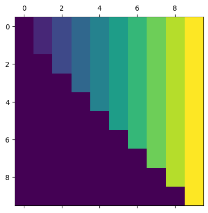 lower triangular matrix ```python print('lower triangular matrix') plt.close() print(np.tril(range(10))) plt.matshow(np.tril(range(10))) plt.show() ``` 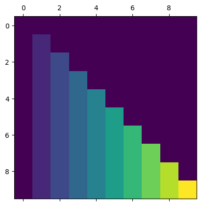 The identity matrix is a square diagonal matrix with all diagonal elements set to 1. Denoted $\mathbf{I}$ or $\mathbf{I}_5$ to indicate a 5x5 matrix. Any matrix of vector times the identity matrix is that same matrix of vector; the identity matrix is the equivalent of the number 1. $$\mathbf{A}\mathbf{I}=\mathbf{I}\mathbf{A}=\mathbf{A}$$ Multiplying by $\mathbf{I}$ leaves the matrix as it is, the way multiplying a number by 1 leaves the number as it is. identity matrix ```python print(np.eye(10)) plt.close() plt.matshow(np.eye(10)) plt.show() ``` 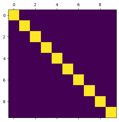 matrix multiplication ```python # Matrix slicing M = np.arange(50).reshape(5,10) # or # mrows = 5 # ncols = 10 # M = np.random.randn(mrows, ncols) submatrix = M[1:4:1, 0:5:1] print('Original matrix:', '\n', M) print('Submatrix:', '\n', submatrix) ``` ```python # matrix multiplication print(M[:5,:5]) plt.close() plt.matshow(M[:5,:5]) plt.show() ``` 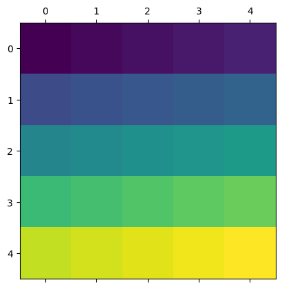 M @ I ```python print(M[:5,:5]@np.eye(5)) plt.close() plt.matshow(M[:5,:5]@np.eye(5)) plt.show() ```  element-wise multiplication ```python # element-wise multiplication print(M[:5,:5]) plt.close() plt.matshow(M[:5,:5]) plt.show() ``` 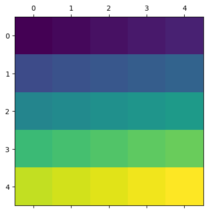 The same matrix element-wise mutliplied by the identity matrix ```python print("The same matrix element-wise mutliplied by the identity matrix") print(M[:5,:5]*np.eye(5)) plt.close() plt.matshow(M[:5,:5]*np.eye(5)) plt.show() ``` 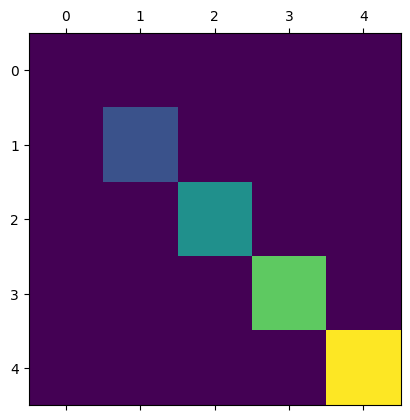 zeros or zero matrix ``` array([[0., 0., 0., 0., 0.], [0., 0., 0., 0., 0.], [0., 0., 0., 0., 0.], [0., 0., 0., 0., 0.], [0., 0., 0., 0., 0.]]) ``` ## Adding and Subtracting Matrices $$ \begin{bmatrix} 0&1&2\\ 0&-1&-2 \end{bmatrix} + \begin{bmatrix} 1 & 2 & 3\\ 4 & 5 & 6 \end{bmatrix} = \begin{bmatrix} (0 + 1) & (1 + 2) & (2+3)\\ (0 + 4) & (-1 + 5) & (-2 + 6) \end{bmatrix} = \begin{bmatrix} 1 & 3 & 5\\ 4 & 4 & 4 \end{bmatrix} $$ add two row vectors ``` a [[ 0 1 2] [ 0 -1 -2]] + b [[1 2 3] [4 5 6]] array([[1, 3, 5], [4, 4, 4]]) ``` add two row vectors ``` a [[ 0 1 2] [ 0 -1 -2]] - b [[1 2 3] [4 5 6]] array([[-1, -1, -1], [-4, -6, -8]]) ``` ## Shifting a Matrix, or adding a scalar It isn't formally possible to add a scalar to a matrix like $\lambda+\mathbf{A}$. Python allows broadcasting a scalar to all the elements of a matrix, like: ```python np.zeros((5,5))+3 ``` ``` array([[3., 3., 3., 3., 3.], [3., 3., 3., 3., 3.], [3., 3., 3., 3., 3.], [3., 3., 3., 3., 3.], [3., 3., 3., 3., 3.]]) ``` In linear algebra, you can *shift* a matrix by adding a constant value to the diagonal, implemented by adding a scalar multiplied identity matrix like $\mathbf{A}+\lambda\mathbf{I}$: $$ \begin{bmatrix} 4 & 5 & 1\\ 0 & 1 & 11\\ 4 & 9 & 7 \end{bmatrix} + 6 \begin{bmatrix} 1 & 0 & 0\\ 0 & 1 & 0\\ 0 & 0 & 1 \end{bmatrix} = \begin{bmatrix} 10 & 5 & 1\\ 0 & 7 & 11\\ 4 & 9 & 13 \end{bmatrix} $$ ```python A = np.array([ [4,5,1],[0,1,11],[4,9,7] ]) s = 6 print(A) print("Not shifting; broadcasting") print(A + s) print("Shifting") print(A + s*np.eye(len(A))) ``` ``` [[ 4 5 1] [ 0 1 11] [ 4 9 7]] Not shifting; broadcasting [[10 11 7] [ 6 7 17] [10 15 13]] Shifting [[10. 5. 1.] [ 0. 7. 11.] [ 4. 9. 13.]] ``` Shifting is the mechanism for finding eigenvalues of a matrix, and regularizing matrices when fitting models to data. An eigenvector is a direction the matrix leaves on the same line. The matrix only stretches it. An eigenvalue is that stretch factor. If $\mathbf{v}$ is such a direction, $\mathbf{v}$ is not the zero vector, and $\lambda$ is the stretch, $$\mathbf{A}\mathbf{v}=\lambda\mathbf{v}$$ Shifting by that $\lambda$ builds $\mathbf{A}-\lambda\mathbf{I}$, which sends that direction to the zero vector. The same kind of shift is what the sentence above calls regularizing: adding a number on the diagonal pulls the matrix toward a multiple of the identity, so a direction that was almost flat gets a definite stretch. The determinant is the single number a square matrix produces, written out in the determinant section below. The values of $\lambda$ that do this are the ones that make $\det(\mathbf{A}-\lambda\mathbf{I})=0$. That equation is the characteristic polynomial, below. ## Scalar and Hadamard Multiplications Both are element-wise operations. **Scalar**: $$ \gamma \begin{bmatrix} a & b\\ c & d \end{bmatrix} = \begin{bmatrix} \gamma a & \gamma b\\ \gamma c & \gamma d \end{bmatrix} $$ **Hadamard**: $$ \begin{bmatrix} 2 & 3\\ 4 & 5 \end{bmatrix} \odot \begin{bmatrix} a & b\\ c & d \end{bmatrix} = \begin{bmatrix} 2a & 3b\\ 4c & 5d \end{bmatrix} $$ scalar multiplication ``` A [[ 4 5 1] [ 0 1 11] [ 4 9 7]] A+6 [[10 11 7] [ 6 7 17] [10 15 13]] ``` hadamard ``` A*B [[ 16 25 1] [ 0 1 121] [ 16 81 49]] np.multiply() [[ 16 25 1] [ 0 1 121] [ 16 81 49]] ``` ## Matrix Multiplication Rather than element-wise, matrix multiplication operates row/column-wise. Standard matrix multiplication reduces to a systematic collection of dot products between rows of one matrix and the columns of the other matrix. **Matrix multiplication is an organized collection of dot products between rows of the left matrix and columns of the right matrix.** ### Rules for MatMul Validity Matrices are written as $M\times N$, rows by columns. Two matrices multiplying each other can have different sizes. So the size of the first matrix is $M \times N$, and the second is $N \times K$. $$ \begin{bmatrix} 0 & 1 & 2\\ 3 & 4 & 5 \end{bmatrix} @ \begin{bmatrix} 0 & 1\\ 2 & 3\\ 4 & 5 \end{bmatrix} $$ $$ M \times N\,@\,N \times K = M \times K $$ If the "inner" dimensions match, the matrix multiplication is valid, and the size of the product is defined by the "outer" dimensions. Put another way, matmul is valid with the number of columns on the left matches the number of rows on the right, and the size of the product is defined by the number of rows on the left, and the number of columns on the right. $$ \begin{bmatrix} 2 & 3\\ 4 & 5 \end{bmatrix} \begin{bmatrix} a & b\\ c & d \end{bmatrix} = \begin{bmatrix} (2a+3c)&(2b+3d)\\ (4a+5c)&(4b+5d) \end{bmatrix} $$ THe dot product is a number that encodes the relationship between two vectors. So, the result of matrix multiplication is a matrix that stores all the pairwise linear relationships between rows of the left matrix and the columns of the right. ```python A = np.array([ [0,1,2],[3,4,5] ]) B = np.array([ [0,1],[2,3],[4,5] ]) C = A@B print("A", A.shape) print(A,'\n') print("B", B.shape) print(B,'\n') print("A@B", C.shape) print(C) ``` ``` A (2, 3) [[0 1 2] [3 4 5]] B (3, 2) [[0 1] [2 3] [4 5]] A@B (2, 2) [[10 13] [28 40]] ``` ## By hand: matrix multiplication @ alan yeh. ai by hand [https://aibyhand.substack.com/](https://aibyhand.substack.com/) [https://aibyhand.substack.com/p/w2-matrix-multiplication](https://aibyhand.substack.com/p/w2-matrix-multiplication) ```python def m(*x): return np.array([[*x]]) def M(*x): return np.array([*x]) ``` ```python # ex1 m(3)@m(5,2) ``` ``` array([[15, 6]]) ``` ```python # ex2 m(3,2).T@m(4) ``` ``` array([[12], [ 8]]) ``` ```python # ex3 m(1,-1).T@m(1,-1) ``` ``` array([[ 1, -1], [-1, 1]]) ``` ```python # ex4 m(3,2).T@m(2,-2) ``` ``` array([[ 6, -6], [ 4, -4]]) ``` ```python # ex5 m(1,0).T@m(3,-5) ``` ``` array([[ 3, -5], [ 0, 0]]) ``` ```python # ex6 m(1,-1).T@m(4,-2) ``` ``` array([[ 4, -2], [-4, 2]]) ``` ```python # ex7 M([1,1],[1,-1])@M([1,3],[3,2]) ``` ``` array([[ 4, 5], [-2, 1]]) ``` ```python # ex8 M([1,1],[1,-1])@M([2,5],[4,3]) ``` ``` array([[ 6, 8], [-2, 2]]) ``` ```python # ex9 M([3,2],[4,5])@M([1,1],[-1,1]) ``` ``` array([[ 1, 5], [-1, 9]]) ``` ```python # ex10 M([5,5],[-2,2])@M([1,1],[-1,1]) ``` ``` array([[ 0, 10], [-4, 0]]) ``` ```python # ex11 M([3,1],[2,4])@M([1,1,-1,-1],[-1,1,1,-1]) ``` ``` array([[ 2, 4, -2, -4], [-2, 6, 2, -6]]) ``` ```python # ex12 M([1,1],[1,-1],[1,0])@M([4,3,2,1],[1,2,1,2]) ``` ``` array([[ 5, 5, 3, 3], [ 3, 1, 1, -1], [ 4, 3, 2, 1]]) ``` ```python # ex13 M([1,0,1],[0,1,1])@M([2,1],[3,5],[4,-1]) ``` ``` array([[6, 0], [7, 4]]) ``` ```python # ex14 M([3,3,-1],[2,1,3])@M([1,1],[1,0],[0,1]) ``` ``` array([[6, 2], [3, 5]]) ``` ```python # ex15 M([1,1],[1,0],[0,1])@M([3,3,-1],[2,1,3]) ``` ``` array([[ 5, 4, 2], [ 3, 3, -1], [ 2, 1, 3]]) ``` ```python # ex16 M([0,1,1],[1,1,0])@M([3,2],[2,1],[1,-2]) ``` ``` array([[ 3, -1], [ 5, 3]]) ``` ```python # ex17 M([1,0,1],[1,1,0])@M([-2,2],[4,4],[3,1]) ``` ``` array([[1, 3], [2, 6]]) ``` ```python # ex18 M([1,1,0,1],[1,0,1,-1])@M([3,2],[2,0],[1,2],[4,3]) ``` ``` array([[9, 5], [0, 1]]) ``` ```python # ex19 M([3,2],[2,0],[1,2],[4,3])@M([1,1,0,1],[1,0,1,-1]) ``` ``` array([[ 5, 3, 2, 1], [ 2, 2, 0, 2], [ 3, 1, 2, -1], [ 7, 4, 3, 1]]) ``` ```python # ex20 M([1,1,0,0],[0,1,1,0],[0,0,1,1],[1,0,0,1])@M([3,2],[2,1],[1,1],[4,3]) ``` ``` array([[5, 3], [3, 2], [5, 4], [7, 5]]) ``` ```python # ex21 M([1,-1,0,0],[0,1,-1,0],[0,0,1,-1],[-1,0,0,1])@M([3,2],[2,1],[1,1],[4,3]) ``` ``` array([[ 1, 1], [ 1, 0], [-3, -2], [ 1, 1]]) ``` ```python # ex22 M([9,-2,0,5],[13,3,1,4])@M([1,0,0,0,1],[0,1,0,0,1],[0,0,1,0,0],[0,0,0,1,0]) ``` ``` array([[ 9, -2, 0, 5, 7], [13, 3, 1, 4, 16]]) ``` ```python # ex23 M([2,-1,1,0],[3,2,4,1])@M([0,0,0,1,1],[1,0,1,0,1],[0,1,1,0,1],[0,1,0,1,0]) ``` ``` array([[-1, 1, 0, 2, 2], [ 2, 5, 6, 4, 9]]) ``` ```python # ex24 M([-1,1,0,0],[0,1,0,0],[-1,0,1,0],[1,0,0,1])@M([3,2],[2,1],[1,1],[4,3]) ``` ``` array([[-1, -1], [ 2, 1], [-2, -1], [ 7, 5]]) ``` ```python # ex25 M([1,1,1,0],[0,1,1,1],[1,0,1,1],[1,1,0,1],[1,1,-1,1])@M([0,0,0,1,1],[1,0,1,0,1],[0,1,1,0,1],[0,0,0,1,0]) ``` ``` array([[ 1, 1, 2, 1, 3], [ 1, 1, 2, 1, 2], [ 0, 1, 1, 2, 2], [ 1, 0, 1, 2, 2], [ 1, -1, 0, 2, 1]]) ``` ## Matrix-vector Multiplication Multiplying a matrix and a vector is not a special operation. The same dimensionality rule applies. ```python A ``` ``` array([[0, 1, 2], [3, 4, 5]]) ``` ```python v = np.array([0,1,2]) # row vector print(A@v) print(A.shape, '@', v.shape) print((A@v).shape) ``` ``` [ 5 14] (2, 3) @ (3,) (2,) ``` Matrix-vector multiplication always results in a vector. The orientation depends on the orientation of the multiplicand vector. ```python v = np.array([[0,1,2]]).T # transposed to columnar print(A@v) print(A.shape, '@', v.shape) print((A@v).shape) ``` ``` [[ 5] [14]] (2, 3) @ (3, 1) (2, 1) ``` ## Matrix-vector Multiplication for Linear Weighted Combinations Put the individual vectors into a matrix, and the weights into the corresponding elements of a vector: $$ 4 \begin{bmatrix} 3\\0\\6 \end{bmatrix} + 3 \begin{bmatrix} 1\\2\\5 \end{bmatrix} \Rightarrow \begin{bmatrix} 3 & 1\\ 0 & 2\\ 6 & 5 \end{bmatrix} \begin{bmatrix} 4\\3 \end{bmatrix} = \begin{bmatrix} (3*4)+(1*3)\\ (0*4)+(2*3)\\ (6*4)+(5*3) \end{bmatrix} = \begin{bmatrix} 15\\6\\39 \end{bmatrix} $$ ```python a = np.array([ [3,0,6],[1,2,5],]) b = np.array([4,3]) a.T@b ``` ``` array([15, 6, 39]) ``` ## By hand: linear layer [https://aibyhand.substack.com/p/w3-linear-layer](https://aibyhand.substack.com/p/w3-linear-layer) ```python def L(w,x): # bias w[:,-1:] # weight w[:,:-1] return w[:,:-1]@x+w[:,-1:] ``` ```python L(M([3,0]), m(4)) ``` ``` array([[12]]) ``` ```python L(M([3,2]), m(4)) ``` ``` array([[14]]) ``` ```python L(M([3,-1]), m(4)) ``` ``` array([[11]]) ``` ```python L(M([3,2],[3,-2]), m(4)) ``` ``` array([[14], [10]]) ``` ```python L(M([3,2],[3,-2],[3,-4]), m(2)) ``` ``` array([[8], [4], [2]]) ``` ```python L(M([1,-1,0]), M([2],[1])) ``` ``` array([[1]]) ``` ```python L(M([2,1,2]), M([2],[3])) ``` ``` array([[9]]) ``` ```python L(M([1,1,0],[1,-1,0]), M([2],[-1])) ``` ``` array([[1], [3]]) ``` ```python L(M([1,1,2],[1,-1,2]), M([2],[1])) ``` ``` array([[5], [3]]) ``` ```python L(M([1,1,0],[0,1,0],[1,-1,0]), M([3],[2])) ``` ``` array([[5], [2], [1]]) ``` ```python L(M([1,1,0],[1,-1,0],[-1,1,0]), M([4],[7])) ``` ``` array([[11], [-3], [ 3]]) ``` ```python L(M([1,-1,1,0],[1,1,1,0]), M([1],[-2],[3])) ``` ``` array([[6], [2]]) ``` ```python L(M([1,1,0,-1],[1,0,1,-1]), M([3],[1],[2])) ``` ``` array([[3], [4]]) ``` ```python L(M([1,1,0,0],[0,1,1,0],[1,0,1,0]), M([3],[1],[2])) ``` ``` array([[4], [3], [5]]) ``` ```python L(M([1,1,0]), M([2],[3])) ``` ``` array([[5]]) ``` ```python L(M([1,0,0]), M([2],[3])) ``` ``` array([[2]]) ``` ```python L(M([1,1,2]), M([2],[1])) ``` ``` array([[5]]) ``` ```python L(M([1,1,-2]), M([2],[1])) ``` ``` array([[1]]) ``` ```python L(M([-1,1,0],[1,-1,0]), M([3],[5])) ``` ``` array([[ 2], [-2]]) ``` ```python L(M([1,2,0],[1,3,0]), M([4],[2])) ``` ``` array([[ 8], [10]]) ``` ```python L(M([1,2,1],[1,2,5]), M([3],[2])) ``` ``` array([[ 8], [12]]) ``` ```python L(M([1,1,0],[2,1,0],[3,0,0]), M([3],[2])) ``` ``` array([[5], [8], [9]]) ``` ```python L(M([1,1,0],[2,1,0],[3,1,0]), M([2],[1])) ``` ``` array([[3], [5], [7]]) ``` ```python L(M([1,1,0,0],[1,1,-1,0],[1,1,1,0]), M([2],[1],[2])) ``` ``` array([[3], [1], [5]]) ``` ```python L(M([1,1,0,0],[1,1,0,-2],[1,1,0,-4]), M([2],[5],[1])) ``` ``` array([[7], [5], [3]]) ``` [https://aibyhand.substack.com/p/w6-batch](https://aibyhand.substack.com/p/w6-batch) ```python L(M([1,1,0,1,0,0,0,0],[1,-1,0,0,0,0,2,0],[-1,0,1,0,1,-1,0,1]), M([2],[1],[3],[1],[2],[1],[1])) ``` ``` array([[4], [3], [3]]) ``` ```python L(M([1,1,0,1,0,0,0,0,0],[1,-1,0,0,0,0,2,-1,0],[-1,0,1,0,1,-1,0,0,1]), M([2],[1],[3],[1],[2],[1],[1],[1])) ``` ``` array([[4], [2], [3]]) ``` ## Geometric Transforms Matrix-vector multiplication is a way of rotating and scaling vectors (scalar-vector multiplication can only scale). ```python M = np.array([ [2,3],[2,1] ]) x = np.array([ [1,1.5] ]).T # composed as a row vector, then transposed Mx = M@x print(Mx) ``` ``` [[6.5] [3.5]] ``` Exposing eigenvalues with geometric transformation ```python # this gets further explained later plt.close() plt.figure(figsize=[6,6]) plt.xlim(-2,8) plt.ylim(-2,8) plt.grid() plt.quiver(0,0,x[0],x[1], angles='xy', scale_units='xy', scale=1) plt.quiver(0,0,Mx[0],Mx[1], angles='xy', scale_units='xy', scale=1) plt.annotate(f"x=({x[0][0]},{x[1][0]})", xy=x, xytext=(3, 3), textcoords="offset points", ha="center") plt.annotate(f"Mx=({Mx[0][0]},{Mx[1][0]})", xy=Mx, xytext=(3, 3), textcoords="offset points", ha="center") plt.title('Exposing eigenvalues with geometric transformation') plt.show() ``` 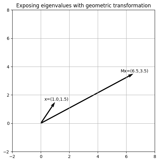 The picture draws $\mathbf{x}$ and $\mathbf{Mx}$ from the code above. An eigenvector would lie on the same line as the arrow it came from, scaled by its eigenvalue. ## Norms Frobenius/Euclidean/l2 norm matrix distance computed as the square root of the sum of the squared elements $$\lVert\mathbf{A}\rVert_F=\sqrt{\sum_i\sum_j a_{ij}^2}$$ Unroll the matrix into one long list of its entries. This is the ordinary vector magnitude of that list: the Pythagorean length in as many dimensions as the matrix has entries. ``` np.float64(10.895423745906376) ``` ## Trace The trace of a matrix is the sum of the diagonal elements. $$\operatorname{tr}(\mathbf{A})=\sum_i a_{ii}$$ The diagonal is the set of entries where the row number equals the column number. ```python np.trace(A) ``` ``` np.int64(14) ``` ```python np.trace(B) ``` ``` np.int64(14) ``` Euclidean/Frobenius norm can also be computed as the square root of the trace of the matrix times its transpose $$\lVert\mathbf{A}\rVert_F=\sqrt{\operatorname{tr}(\mathbf{A}^\top\mathbf{A})}$$ The product $\mathbf{A}^\top\mathbf{A}$ places, on its diagonal, the squared length of each column. The trace adds those diagonal entries, which adds the square of every entry of $\mathbf{A}$, and the square root is the Frobenius length above. ``` 21.142374511865974 21.142374511865974 ``` ## Matrix Space There are 4 matrix spaces: column, row, null, left-null. They are defined as the set of linear weighted combinations of different features of the matrix. - Column space comprises all the linear weighted combinations of the columns in the matrix and is written $C(\mathbf{A})$. - Row space comprises all the linear weighted combinations of the rows in the matrix and is written $R(\mathbf{A})$ or $C(\mathbf{A}^T)$. ## Null Space Null space is the set of non-trivial vectors such that, given a matrix $\mathbf{A}$ and a vector $\mathbf{y}$, $\mathbf{Ay}=\mathbf{0}$. It is the set of vectors that linearly combines the columns to produce the zeros vector--in other words, any vector $\mathbf{y}$ that solves the equation $\mathbf{Ay}=\mathbf{0}$. The trivial solution $\mathbf{y}=\mathbf{0}$ is excluded. The null space is important for finding eigenvectors and other things. The left null space is the same idea applied on the left. It is the set of row vectors $\mathbf{y}^\top$ such that $\mathbf{y}^\top\mathbf{A}=\mathbf{0}$, which is the null space of $\mathbf{A}^\top$. Full-rank and full column-rank matrices have empty null spaces, whereas reduced-rank matrices have nonempty(nontrivial) null spaces. The null space is empty when the columns of the matrix form a linearly independent set. A is a reduced-rank matrix and so has a non-trivial null space. ``` matrix A: [[ 1 -1] [-2 2]] rank: 1 null space: [[ 0.70710678 -0.70710678] [-1.41421356 1.41421356]] ``` B is a full-rank matrix and so it's null space is an empty set thus, the code fails ``` matrix A: [[ 1 -1] [-2 3]] rank: 2 Failed to calculate nullspace because operands could not be broadcast together with shapes (2,2) (2,0) ``` ## Rank Rank is a non-negative integer associated with a matrix. It reflects the largest number of columns (or rows) that can form a linearly independent set. Matrices with a rank smaller than the maximum possible are called reduced-rank or singular. The rank of a matrix is the dimension of the vector space generated by its columns. The vector space is described by the set of possible vectors in the matrix, and if vector $\mathbf{a}$ can be described as the linear combination of vector $\mathbf{b}$, then they are part of the same subspace. Rank-nullity ties rank to the null space. If $\mathbf{A}$ has $n$ columns, $$\operatorname{rank}(\mathbf{A})+\dim N(\mathbf{A})=n$$ Rank counts how many independent directions survive the multiplication. $\dim N(\mathbf{A})$ counts how many independent directions collapse to the zero vector. Dimension here means how many independent vectors it takes to build that set. ### Reduced Rank A matrix is reduced-rank if at least one column can be expressed as a linear combination of other columns. Max rank is the smaller of its row or column count i.e. Max rank = min{M,N} TODO: Add check for linear independence first because vectors must be linearly independent ``` Rank: 2 Rank: 6 Np rank: 2 Np rank: 6 ``` matrix augmentation transpose into a column vector ``` array([[1], [2], [3]]) matrix([[4, 5, 6, 1], [0, 1, 2, 2], [9, 9, 4, 3]]) ``` matrix augmentation a second way transpose into a column vector ``` array([[1], [2], [3]]) matrix([[4, 5, 6, 1], [0, 1, 2, 2], [9, 9, 4, 3]]) ``` ## Determine if a Vector is in Matrix Column Space 1. **Augment the matrix with the vector**. The original matrix is $\mathbf{A}$, and the augmented matrix is $\mathbf{\widetilde{A}}$. 2. **Compute the ranks of the two matrices**. 3. **Compare the two ranks**. There will be one of two possible outcomes: - $rank(\mathbf{A})=rank(\mathbf{\widetilde{A}})$. Vector $\mathbf{v}$ is in the column space of matrix $\mathbf{A}$. - $rank(\mathbf{A})<rank(\mathbf{\widetilde{A}})$. Vector $\mathbf{v}$ is **not** in the column space of matrix $\mathbf{A}$. If $\mathbf{v}\in C(\mathbf{A})$, then $\mathbf{v}$ can be expressed as some linear weighted combination of the columns of $\mathbf{A}$. The columns of the augmented matrix $\widetilde{\mathbf{A}}$ form a linearly dependent set. In terms of span, vector $\mathbf{v}$ is redundant in $\widetilde{\mathbf{A}}$. Hence, rank remains the same. Conversely, if $\mathbf{v}\notin C(\mathbf{A})$, then $\mathbf{v}$ cannot be expressed as a linear weighted combination of the columns of $\mathbf{A}$, which means that $\mathbf{v}$ has added new inforrmation into $\widetilde{\mathbf{A}}$. And that means the rank will increase by 1. ## Determining Linear Independence of a Vector Set place vectors in a matrix compute the rank of the matrix compare that rank to the maximum possible rank of that matrix: min(M,N). possible outcomes: r = M: The vector set is linearly independent. r < M: The vector set is linearly dependent. ``` Dependent ``` place vectors in a matrix compute the rank of the matrix compare that rank to the maximum possible rank of that matrix: min(M,N). possible outcomes: r = M: The vector set is linearly independent. r < M: The vector set is linearly dependent. ``` Independent ``` If the rank is smaller than the number of columns, then at least one column can be described as a linear combination of the other columns. If the rank equals the number of columns, then each column contributes unique information to the matrix, which means that no column can be described as a linear combination of others. ## Determinant Denoted $det(\mathbf{A})$ or $|\mathbf{A}|$. Greek capital delta $\Delta$ can be used when not referring to a specific matrix. For a 2 by 2 matrix the determinant is one product minus the other: $$\det\begin{bmatrix}a & b \\ c & d\end{bmatrix}=ad-bc$$ That number is the signed area of the parallelogram spanned by the two columns. A parallelogram is a pushed rectangle: opposite sides stay parallel. Signed means a negative value is that same area with the columns swapped, a flip. In more dimensions the determinant is the signed volume of the box the columns span. Zero means the box has been flattened, which is the reduced-rank case below. My book by Mike Cohen suggests computing the determinant is an awful experience and "if I live a thousand years" without doing it by hand it will be worth it. I read his quick explanation of why this is true, and can verify I won't even be attempting it. I get it, it's horrific and onerous and it's 2024 so let's come back to that when we have time and money in surplus. `np.linalg.det()` or `scipy.linalg.det()` will do nicely. **Note, the determinant is done on a square matrix.** Reduced-rank matrices have a determinant $\Delta=0$. Full-rank matrices have a non-zero determinant $\Delta\ne 0$. This is because the determinant represents the scaling factor of a volume in the matrix space when a linear transformation is applied by the matrix. Only square matrices can represent linear transformations that map a vector space to itself, which is necessary for the determinant to be defined. For example, a 1x1 space is transformed by a square matrix. The volume of that 1x1 space, when transformed by a square matrix, is scaled by the determinant of the matrix. $\Delta=0$ can be geometrically interpreted as a matrix transformation in which at least one dimension gets flattened to have a surface area but no volume. This is because the determinant is the volume of the transformed space, and if the determinant is 0, then the volume of the transformed space is 0. ```python # plot a transformation XMIN, XMAX, YMIN, YMAX = -2, 2, -2, 2 N = 16 xgrid = np.linspace(XMIN, XMAX, N) ygrid = np.linspace(YMIN, YMAX, N) grid = np.array(np.meshgrid(xgrid, ygrid)).reshape(2, N**2) basis = np.array([[1,0], [0,1]]) plt.scatter(*grid, color="k", s=2, alpha=0.5) ix, iy = basis[0] jx, jy = basis[1] plt.plot([0, ix, ix+jx, jx, 0], [0, iy, iy+jy, jy, 0], color="k") plt.axis("square") plt.show() ``` 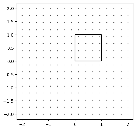 in this example, a space is transformed by a 5x5 matrix, and the determinant shows that the volume of the space is scaled by the determinant factor. ``` 6.0 ``` this matrix is reduced-rank because the vectors are linearly dependent. this has the effect of collapsing the volume of the space to 0, because some of the vectors lie along the same line. ``` 0.0 ``` ## Characteristic Polynomial Combining shifting a matrix with the determinant is called the *characteristic polynomial*. $$det(\mathbf{A}-\lambda\mathbf{I})=\Delta$$ It transforms a square matrix, shifted by $\lambda$, into an equation that equals the determinant. Knowing the determinant allows you to solve for $\lambda$. The eigenvalues are the values of $\lambda$ that make $\det(\mathbf{A}-\lambda\mathbf{I})=0$. Those are the stretches $\mathbf{A}\mathbf{v}=\lambda\mathbf{v}$ from the shifting section. The line above sets the shifted determinant equal to $\Delta$. Setting that determinant equal to zero, and expanding, produces the polynomial whose roots are the eigenvalues. A root is a number that makes the polynomial equal zero. ```python A ``` ``` matrix([[1, 3], [3, 1]]) ``` ```python print("The shifted matrix.") print(A - I) ``` ``` The shifted matrix. [[3. 3.] [3. 3.]] ``` ```python print("The characteristic polynomial", np.linalg.det(A-I)) ``` ``` The characteristic polynomial 0.0 ``` Next: [Matrix applications](matrix-applications.html).