Matrix applications Covariance is the dot product between two mean-centered variables. math · matrices Study sequence: [Vectors](vectors.html) · [Matrices](matrices.html) · Matrix applications · [Calculus](calculus.html) · [Big O](big-o.html) · [Geometry](geometry.html) · [Signals](signals.html) · [Neural nets](neural-nets.html) · [Distributions](distributions.html) # Matrix Applications ## Multivariate Data Covariance Matrices Covariance is interpreted the same as correlation: when variables move together it is positive, negative when they move apart, and 0 if there is no linear relationship. That's because covariance is the dot product between two mean-centered variables. It's the numerator of the [Pearson correlation coefficient](vectors.html#pearson-correlation-coefficient): $$c_{a,b} = (n-1)^{-1}\sum^n_{i=1}(x_i - \bar{x})(y_i - \bar{y})$$ $x^{-1}=\frac{1}{x}$. And, as in the Pearson correlation coefficient, if $\mathbf{\widetilde{x}}$ is the mean-centered variable $\mathbf{x}$, and $$\mathbf{\widetilde{x}}^\text{T}\mathbf{\widetilde{y}}\frac{1}{n-1}$$ then covariance is simply $$\frac{\mathbf{\widetilde{x}}^\text{T}\mathbf{\widetilde{y}}}{n-1}$$ Covariance has a normalization factor of $n-1$, where n is the number of data points. Normalization prevents the covariance from growing larger as you sum more data values together. It's analogous to dividing by $N$ to transform a sum into an average. The centering step, worked by hand, is in [Vectors](vectors.html#by-hand-mean-centering). blur around centroid (std units) ```python ## Create data nPerClust = 50 # blur around centroid (std units) blur = 1 # XY centroid locations A = [ 1, 1 ] B = [ -3, 1 ] C = [ 3, 3 ] # generate data a = [ A[0]+np.random.randn(nPerClust)*blur , A[1]+np.random.randn(nPerClust)*blur ] b = [ B[0]+np.random.randn(nPerClust)*blur , B[1]+np.random.randn(nPerClust)*blur ] c = [ C[0]+np.random.randn(nPerClust)*blur , C[1]+np.random.randn(nPerClust)*blur ] # concatenate into a matrix df = pd.DataFrame(np.transpose(np.concatenate((a,b,c),axis=1))) plt.close() display(df.T.cov()) plt.matshow(df.T.cov()) plt.colorbar(shrink=0.7) plt.show() # Unsurprising that the covariance of normally # distributed variables look normally distributed. ``` 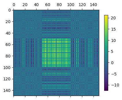 databetes dataset feature covariance ```python # using the sklearn diabetes dataset # note the similarities between # correlation and covariance from sklearn.datasets import load_diabetes data = load_diabetes() feature_names = data['feature_names'] plt.close() df = pd.DataFrame(data['data']).cov() df.columns = feature_names df.index = feature_names img = plt.matshow(df) plt.title("databetes dataset feature covariance") cbar = plt.colorbar(img, shrink=0.8, label="covariance") plt.grid(color="black") plt.xticks(ticks=[i for i in range(10)], labels=feature_names, fontsize="small") plt.yticks(ticks=[i for i in range(10)], labels=feature_names, fontsize="small") plt.show() display("Covariance", df) display("Pearson Correlation", df.corr()) ``` 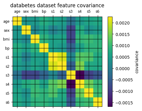 Note that the correlation and covariance matrices are similar, except that the scales are different. This is because covariance ```python # Note that the correlation and covariance matrices are similar, # except that the scales are different. This is because covariance # retains the scale of the original data, and so is not bound to [-1,1]. plt.close() fig, axs = plt.subplots(nrows=1, ncols=2) fig.subplots_adjust(left=1.0, right=2.5) cov = axs[0].matshow(df) fig.colorbar(cov, ax=axs[0], shrink=0.94) axs[0].set_title("covariance") cor = axs[1].matshow(df.corr()) fig.colorbar(cor, ax=axs[1], shrink=0.94) axs[1].set_title("correlation") plt.show() ``` 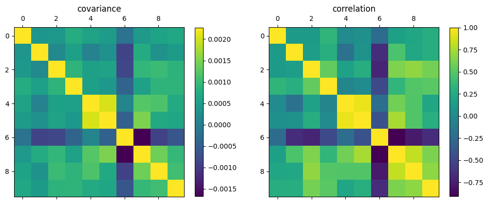 manually calculated covariance ```python # a manual covariance matrix means = np.mean(df, axis=0) # the vector of feature means mean_centered_data = df - means covariance_matrix = mean_centered_data.T @ mean_centered_data covariance_matrix /= (mean_centered_data.shape[0]-1) # divided by n-1 plt.close() plt.matshow(covariance_matrix) plt.title("manually calculated covariance") ``` 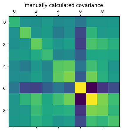 ## Geometric Transformations via Matrix-Vector Multiplication Pure rotation matrices are used to rotate a vector while preserving its length. A 2D rotation matrix can be expressed as: $$ \mathbf{T}= \begin{bmatrix} \cos(\theta) & \sin(\theta) \\ -\sin(\theta) & \cos(\theta) \end{bmatrix} $$ A pure rotation matrix is orthogonal. The columns of $\mathbf{T}$ are orthogonal because their dot product is $\cos(\theta)\sin(\theta)-\sin(\theta)\cos(\theta)$, and are unit vectors because of the Pythagorean trigonometric identity that $\cos^2(\theta)+sin^2(\theta)=1$. dot products of different angles for the rotation matrix a 0 dot product means the vectors are orthogonal ``` [np.float64(0.0), np.float64(0.0), np.float64(0.0), np.float64(0.0), np.float64(0.0), np.float64(0.0), np.float64(0.0)] ``` Pythagorean trig identity of different angles ``` [np.float64(1.0), np.float64(1.0), np.float64(1.0), np.float64(0.9999999999999999), np.float64(1.0), np.float64(0.9999999999999999), np.float64(0.9999999999999999)] ``` To use the transformation matrix $\mathbf{T}$, set $\theta$ to some angle of clockwise rotation, and multiply matrix $\mathbf{T}$ by a 2 x *N* matrix of geometric points, where each column in that matrix contains the (X,Y) coordinates for each of N data points. Geometric transformation of a matrix ```python Y = np.linspace(-5, 5, 20) X = np.array([0]*20) v1 = np.array([X,Y]) theta = np.pi/5 # a positive rotation T = np.array([ [np.cos(theta), np.sin(theta)], [-np.sin(theta), np.cos(theta)] ]) # a negative rotation negT = np.array([ [np.cos(theta), np.sin(theta)], [np.sin(theta), -np.cos(theta)] ]) v2 = T @ v1 v3 = negT @ v1 plt.close() plt.plot(v1[0], v1[1], "o", label="original") plt.plot(v2[0], v2[1], "o", label="rotated") plt.plot(v3[0], v3[1], "o", label="negative rotated") plt.legend() plt.grid() plt.title("Geometric transformation of a matrix") ```  Geometric rotations are transformations, so you can also stretch or scale. In general, the diagonal elements scale the x-axis and y-axis coordinates, while the off-diagonal elements stretch both axes. Geometric transformation of a matrix ```python Y = np.linspace(-5, 5, 20) X = np.array([0]*20) v1 = np.array([X,Y]) theta = np.pi/5 T = np.array([ [5, 0], [0, 5] ]) v2 = T @ v1 plt.close() plt.plot(v2[0], v2[1], "o", label="transformed") plt.plot(v1[0], v1[1], "o", label="original") plt.legend() plt.grid() plt.title("Geometric transformation of a matrix") ```  apply the transformation to the points using matrix multiplication update the dots ```python # Ref: https://github.com/mikexcohen/LinAlg4DataScience/blob/main/LA4DS_ch07.ipynb import matplotlib.animation as animation from matplotlib import rc rc('animation', html='jshtml') # function to update the axis on each iteration def aframe(ph): # create the transformation matrix T = np.array([ [ 1, 1-ph ], [ 0, 1 ] ]) # apply the transformation to the points using matrix multiplication P = T@points # update the dots plth.set_xdata(P[0,:]) plth.set_ydata(P[1,:]) # export the plot handles return plth # define XY points theta = np.linspace(0,2*np.pi,100) points = np.vstack((np.sin(theta),np.cos(theta))) # setup figure fig,ax = plt.subplots(1,figsize=(12,6)) plth, = ax.plot(np.cos(x),np.sin(x),'ko') ax.set_aspect('equal') ax.set_xlim([-2,2]) ax.set_ylim([-2,2]) # define values for transformation (note: clip off the final point for a smooth animation loop) phi = np.linspace(-1,1-1/40,40)**2 # run animation! animation.FuncAnimation(fig, aframe, phi, interval=100, repeat=True) ```  ## Image Feature Detection with Convolution First we design a 2D gaussian kernel. The equation is: $$G=exp(-(X^2+Y^2)/\sigma)$$ This is the same as: $$G=e^{(-(X^2+Y^2)/\sigma)}$$ Where $X$ and $Y$ are 2D grids of (x,y) coordinates on which to evaluate the function, $\sigma$ is a parameter of the function called the "shape" or "width": smaller values make the Gaussian narrower, while larger values make it wider. $X^2+Y^2$ is the squared straight-line distance from the middle of the grid. It is the Pythagorean sum of one horizontal step and one vertical step. The exponential of the negative of that distance is tall at the center and falls toward the corners. normalize the kernel sum to 1 during matmul it preserves the data scale Gaussian parameters ```python def gaussian(size=21, sigma=5): xs = np.linspace(-3,3,size) X,Y = np.meshgrid(xs,xs) kernel = np.exp(-(X**2+Y**2)/sigma) # normalize the kernel sum to 1 # during matmul it preserves the data scale kernel = kernel / np.sum(kernel) return kernel ``` ```python print("Gaussian parameters") plt.close() fig, axs = plt.subplots(ncols=4, figsize=[10,5]) axs[0].matshow(gaussian(21,5)) axs[1].matshow(gaussian(21,10)) axs[2].matshow(gaussian(21,15)) axs[3].matshow(gaussian(21,20)) axs[0].set_title("size:21, sigma:5") axs[1].set_title("size:21, sigma:10") axs[2].set_title("size:21, sigma:15") axs[3].set_title("size:21, sigma:20") plt.show() ```  Gaussian parameters ```python print("Gaussian parameters") plt.close() fig, axs = plt.subplots(ncols=4, figsize=[10,5]) axs[0].matshow(gaussian(5,5)) axs[1].matshow(gaussian(10,5)) axs[2].matshow(gaussian(15,5)) axs[3].matshow(gaussian(21,5)) axs[0].set_title("size:5, sigma:5") axs[1].set_title("size:10, sigma:5") axs[2].set_title("size:15, sigma:5") axs[3].set_title("size:21, sigma:5") plt.show() ``` 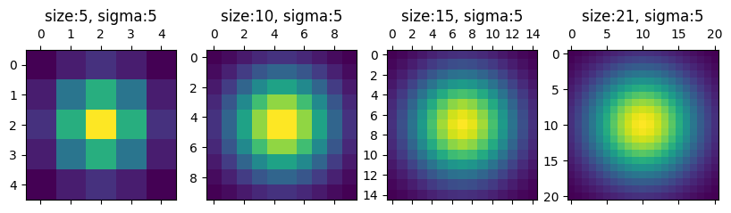 ```python plt.close() plt.matshow(gaussian(1001,3)) plt.colorbar(shrink=0.8) plt.show() ``` 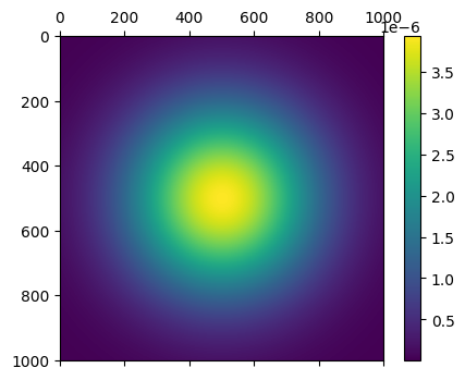 ```python from sklearn.datasets import load_sample_image china = load_sample_image('china.jpg') print("image shape:", china.shape) plt.close() plt.imshow(china) plt.show() ``` 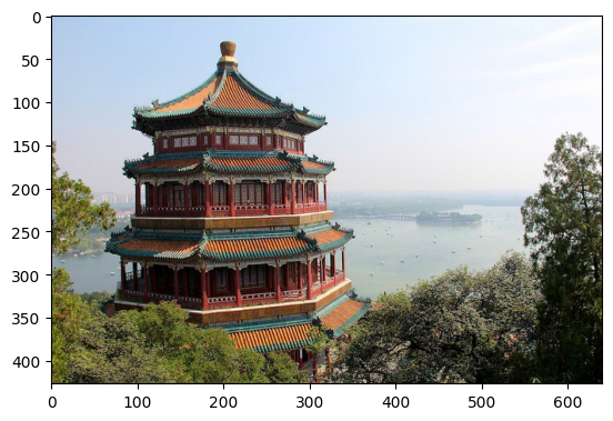 to use a guassian kernel to convolve the image of china first, we must remove separate the color channels to make the ```python # to use a guassian kernel to convolve the image of china # first, we must remove separate the color channels to make the # array two dimensional, then use scipy's convolve implementation # which is computationally superior to a manual nested loop. # it does so by leveraging convolution theory, and applies # the convolution in the frequency domain, rather than the # time/space domain, because convolution in time/space domain # equals multiplication in the frequency domain. this is especially # true as the image grows in size, because there are likely fewer # frequency bins than pixels. we also process each color channel # individually because the convolution function is for 2D images. # we then combine the images together to reform the color channels. kernel = gaussian(50,3) convolution_channel0 = scipy.signal.convolve2d(china[:,:,0], kernel, boundary="symm") convolution_channel1 = scipy.signal.convolve2d(china[:,:,1], kernel, boundary="symm") convolution_channel2 = scipy.signal.convolve2d(china[:,:,2], kernel, boundary="symm") plt.close() fig, axs = plt.subplots(ncols=3, figsize=[15,10]) axs[0].imshow(convolution_channel0, cmap="grey") axs[1].imshow(convolution_channel1, cmap="grey") axs[2].imshow(convolution_channel2, cmap="grey") plt.show() ``` 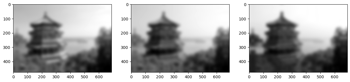 the shape of the original image height x width x color ``` (427, 640, 3) ``` the convolved images, combined together in an array ``` (3, 476, 689) ``` move the axes around so that the color channel is last ``` (476, 689, 3) ``` the convolution changes all the RGB values to floats they must either be normalized to float[0,1] or int[0,255] ```python # the convolution changes all the RGB values to floats # they must either be normalized to float[0,1] or int[0,255] convoluted_color_img = np.moveaxis(color,0,-1).astype("int") plt.close() plt.imshow(convoluted_color_img) plt.show() ``` 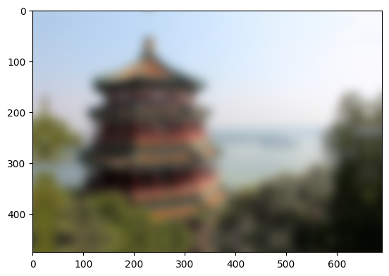 The convolution process is the same as used in [Signal smoothing with a kernel and dot product](vectors.html#signal-smoothing-with-a-kernel-and-dot-product); Hadamard multiply and then sum to retrieve the dot products. The only difference is that it is done on two dimensions instead of one. In one dimension the sum, with the kernel flipped as it slides, is $$(f*g)[n]=\sum_k f[k]\,g[n-k]$$ The index $n-k$ runs the kernel backwards while $n$ says where the window sits. In two dimensions the same sum runs over rows and over columns. The Gaussian kernel above is one such window. vertical edge detection with a vertical kernel ```python # vertical edge detection # with a vertical kernel vertical_kernel = np.array([ [-1, 0, 1], [-1, 0, 1], [-1, 0, 1], ]) convolution_channel0 = scipy.signal.convolve2d(china[:,:,0], vertical_kernel, boundary="symm") convolution_channel1 = scipy.signal.convolve2d(china[:,:,1], vertical_kernel, boundary="symm") convolution_channel2 = scipy.signal.convolve2d(china[:,:,2], vertical_kernel, boundary="symm") color = np.array([ np.clip(convolution_channel0, 0, 255), # clip values to the RGB integer range np.clip(convolution_channel1, 0, 255), np.clip(convolution_channel2, 0, 255) ]) np.moveaxis(color,0,-1).shape vertical_convoluted_color_img = np.moveaxis(color,0,-1).astype("int") plt.close() plt.imshow(vertical_convoluted_color_img) plt.show() ``` 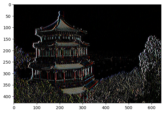 horizontal edge detection with a horizontal kernel ```python # horizontal edge detection # with a horizontal kernel horizontal_kernel = np.array([ [-1, -1, -1], [0, 0, 0], [1, 1, 1], ]) convolution_channel0 = scipy.signal.convolve2d(china[:,:,0], horizontal_kernel, boundary="symm") convolution_channel1 = scipy.signal.convolve2d(china[:,:,1], horizontal_kernel, boundary="symm") convolution_channel2 = scipy.signal.convolve2d(china[:,:,2], horizontal_kernel, boundary="symm") color = np.array([ np.clip(convolution_channel0, 0, 255), np.clip(convolution_channel1, 0, 255), np.clip(convolution_channel2, 0 ,255) ]) np.moveaxis(color,0,-1).shape horizontal_convoluted_color_img = np.moveaxis(color,0,-1).astype("int") plt.close() plt.imshow(horizontal_convoluted_color_img) plt.show() ``` 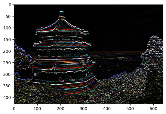 convolution can be used to compress image data once the edges have been detected, many of the ```python # convolution can be used to compress image data # once the edges have been detected, many of the # color values have been eliminated while leaving # the image identifiable. plt.imshow(np.clip(vertical_convoluted_color_img*horizontal_convoluted_color_img, 0, 255)) plt.show() ``` 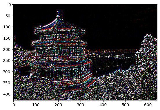 ## The Matrix Equation Ax=b If $\mathbf{A}$ is an $m\times n$ matrix, with columns $\mathbf{a}_1,\dots,\mathbf{a}_n$, and if $\mathbf{x}$ is in $\mathbb{R}^n$, then the product of $\mathbf{A}$ and $\mathbf{x}$ is denoted by $\mathbf{Ax}$, is the linear combination of the columns of $\mathbf{A}$ using the corresponding entries in $\mathbf{x}$ as weights: $$ \mathbf{Ax}= \begin{bmatrix}\mathbf{a}_1&\mathbf{a}_2&\dots&\mathbf{a}_n \end{bmatrix} \begin{bmatrix} x_1\\x_2\\\vdots\\x_n \end{bmatrix} = x_1\mathbf{a}_1 + x_2\mathbf{a}_2+\dots+x_n\mathbf{a}_n $$ and can only be valid if the number of columns in $\mathbf{A}$ equals the number of entries in $\mathbf{x}$. ## Matrix Inversion The inverse of matrix $\mathbf{A}$ is matrix $\mathbf{A}^{-1}$ ("A inverse"). We use it to solve $\mathbf{Ax}=\mathbf{b}$ when $\mathbf{A}$ and $\mathbf{b}$ are known and we want to solve for $\mathbf{x}$. The solution is generally: $$ \begin{align} \mathbf{Ax}&=\mathbf{b} \\ \mathbf{A^{-1}Ax}&=\mathbf{A^{-1}b} \\ \mathbf{Ix}&=\mathbf{A^{-1}b}\\ \mathbf{x}&=\mathbf{A^{-1}b} \end{align} $$ Types of Inverses ### Full Inverse Only square, full-rank matrices can have a full inverse. This means that, for square, full-rank matrices $\mathbf{A^{-1}A}=\mathbf{AA^{-1}}=\mathbf{I}$. ### One-sided Inverse A tall matrix $\mathbf{T}$ can have a *left-inverse*: $\mathbf{LT}=\mathbf{I}$ but $\mathbf{TL}\ne\mathbf{I}$, and if it is full rank-*N* (full column rank). A wide matrix $\mathbf{W}$ can have a *right-inverse*: $\mathbf{WR}=\mathbf{I}$ but $\mathbf{RW}\ne\mathbf{I}$, and if it is full rank-*M* (full row rank). ### Pseudoinverse All full-rank matrices have pseudoinverse matrices which are the same as full and one-sided intverted matrices respectively. But reduced-rank matrices have a pseudoinverse matrix which is close, but not equal, to the identity matrix. These are called *singular* or *noninvertible*, which is pseudonymous with *reduced-rank* or *rank-deficient*. ### Computing the Left-Inverse and Application Producing the identity matrix, the next 4 steps, follow the equation: $$(\mathbf{T}^\text{T}\mathbf{T})^{-1}(\mathbf{T}^\text{T}\mathbf{T})=\mathbf{I}$$ In order to produce the identity matrix for $\mathbf{T}$ we use the inverse of $(\mathbf{T}^{\text{T}}\mathbf{T})$, thus we're not using the inverse of $\mathbf{T}$. Then we multiply the inverse matrix by the transposed matrix $\mathbf{T}$: $$\begin{align} \mathbf{L}&=(\mathbf{T}^{\text{T}}\mathbf{T})^{-1}\mathbf{T}^{\text{T}} \\ \mathbf{LT}&=\mathbf{I} \end{align} $$ generate a tall matrix ```python T = np.random.randint(-10,11,size=(40,4)) # generate a tall matrix plt.close() plt.matshow(T) plt.show() ```  T.T @ T produces a full-rank matrix because T is full column rank, and all full rank matrices have an inverse ```python # T.T @ T produces a full-rank matrix # because T is full column rank, and # all full rank matrices have an inverse TatT = T.T @ T # compute the inverse TatT_inv = np.linalg.inv(TatT) # demonstrate that T.T@T @ T.T@T**-1 # produces the identity matrix I = TatT_inv @ TatT plt.close() fig, axs = plt.subplots(ncols=3) axs[0].matshow(TatT) axs[1].matshow(TatT_inv) axs[2].matshow(I) plt.show() ``` 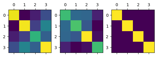 produce the left inverse by matmul T.T@T**-1 @ T.T ```python # produce the left inverse by matmul T.T@T**-1 @ T.T L = TatT_inv @ T.T plt.close() plt.matshow(L) plt.show() ```  matmul the left inverse by T ```python # matmul the left inverse by T TatL = T@L plt.close() plt.matshow(TatL) plt.show() ``` 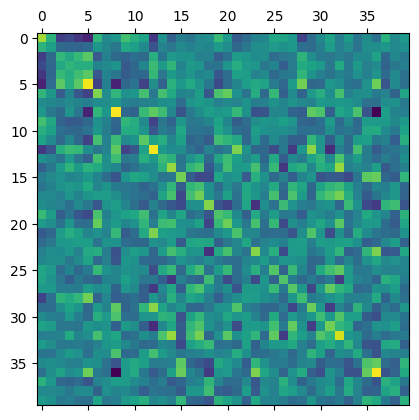 The matrix inverse is unique; if a matrix has an inverse, it has exactly one. There cannot be two matrices $\mathbf{B}$ and $\mathbf{C}$ such that $\mathbf{AB}=\mathbf{I}$ and $\mathbf{AC}=\mathbf{I}$ if $\mathbf{B}\ne\mathbf{C}$. ## Moore-Penrose Pseudoinverse Reduced-rank matrices cannot be transformed into the identity matrix via matrix multiplication, meaning they have no full or one-sided inverse. But singular matrices do have pseudoinverses. Pseudoinverses are transformation matrices that bring a matrix close to the identity matrix. A reduced-rank matrix has an infinite number of pseudoinverses. The Moore-Penrose pseudoinverse, *MP* pseudoinverse, is the most common and the one generally referred to. Denoted with dagger, plus, or asterisk in superscript: $\mathbf{A}^\dagger$, $\mathbf{A}^+$, or $\mathbf{A}^*$. $$ \begin{align} \begin{bmatrix} 1 & 4\\ 2 & 8 \end{bmatrix} &=\frac{1}{85} \begin{bmatrix} 1 & 2\\ 4 & 8 \end{bmatrix} \\ \begin{bmatrix} 1 & 4\\ 2 & 8 \end{bmatrix} \frac{1}{85} \begin{bmatrix} 1 & 2\\ 4 & 8 \end{bmatrix} &= \begin{bmatrix} .2 & .4\\ .4 & .8 \end{bmatrix} \end{align} $$ ```python A = np.array([ [1,4], [2,8] ]) A_pinv = np.linalg.pinv(A) A@A_pinv ``` ``` array([[0.2, 0.4], [0.4, 0.8]]) ``` To compute the MP pseudoinverse take the singular value decomposition of a matrix, invert the nonzero singular values without changing the singular vectors, and reconstruct the matrix by multiplying $\mathbf{U\Sigma^+V^\text{T}}$. Singular value decomposition splits a matrix into three factors: $$\mathbf{A}=\mathbf{U}\boldsymbol{\Sigma}\mathbf{V}^\top$$ The columns of $\mathbf{U}$ and of $\mathbf{V}$ are orthogonal and of length 1, so each of those matrices is a rotation, a turn that keeps lengths. $\boldsymbol{\Sigma}$ is diagonal: entries off the diagonal, where the row number differs from the column number, are zero. The diagonal entries are the singular values, the stretch factors, written $\sigma$. The pseudoinverse keeps the rotations and replaces each nonzero stretch $\sigma$ with $1/\sigma$, and leaves the zeros as zeros. When $\mathbf{A}$ is square and full rank, every stretch is nonzero, and this product is the ordinary inverse. ## Orthogonality Orthogonal Vectors ```python import numpy as np import matplotlib.pyplot as plt # Simplest orthogonal vectors in 2D v1 = np.array([1, 0]) # points right v2 = np.array([0, 1]) # points up # Verify orthogonality (dot product should be 0) dot_product = np.dot(v1, v2) print(f"Dot product: {dot_product}") # Should be 0 # Visualization def plot_vectors(): plt.figure(figsize=(6, 6)) plt.axhline(y=0, color='k', linestyle='-', alpha=0.3) plt.axvline(x=0, color='k', linestyle='-', alpha=0.3) # Plot vectors plt.quiver([0, 0], [0, 0], [v1[0], v2[0]], [v1[1], v2[1]], angles='xy', scale_units='xy', scale=1) plt.xlim(-1.5, 1.5) plt.ylim(-1.5, 1.5) plt.grid(True) plt.title("Orthogonal Vectors") plt.show() plot_vectors() ``` 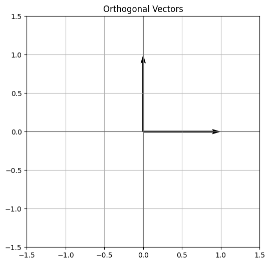 2x2 orthogonal matrix (rotation matrix) Verify orthogonality properties Property 1: Columns are orthogonal Property 2: Transpose = Inverse ``` Rotation Matrix: [[ 0.70710678 -0.70710678] [ 0.70710678 0.70710678]] Dot product of columns: -1.0146536357569526e-17 Matrix * Matrix^T: [[1. 0.] [0. 1.]] ``` Those two properties are one equation. For a square matrix $\mathbf{Q}$ whose columns are orthogonal and of length 1, $$\mathbf{Q}^\top\mathbf{Q}=\mathbf{I}$$ so the inverse is the transpose, $\mathbf{Q}^{-1}=\mathbf{Q}^\top$. A rotation turns vectors and keeps their lengths, which is why distances survive the multiplication. Three mutually orthogonal vectors (standard basis) Verify all pairs are orthogonal ``` 3D Orthogonality Check: v1 · v2 = 0 v2 · v3 = 0 v1 · v3 = 0 ``` RGB basis vectors are orthogonal ```python # RGB basis vectors are orthogonal red = np.array([1, 0, 0]) green = np.array([0, 1, 0]) blue = np.array([0, 0, 1]) def visualize_rgb(): fig = plt.figure(figsize=(8, 8)) ax = fig.add_subplot(111, projection='3d') # Plot vectors ax.quiver(0, 0, 0, red[0], red[1], red[2], color='r') ax.quiver(0, 0, 0, green[0], green[1], green[2], color='g') ax.quiver(0, 0, 0, blue[0], blue[1], blue[2], color='b') ax.set_xlabel('X') ax.set_ylabel('Y') ax.set_zlabel('Z') ax.set_title('RGB Color Space Basis Vectors') plt.show() visualize_rgb() ``` 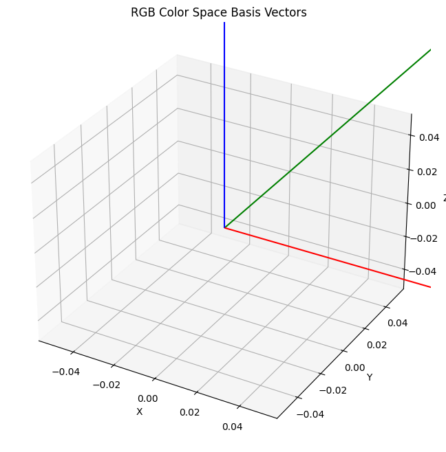 Test these properties 1. Columns orthogonal 2. Preserves distances ``` Columns orthogonal: True Original length: 1.4142135623730951 Transformed length: 1.414213562373095 ``` 90° Rotation Matrix Properties ```python import numpy as np import matplotlib.pyplot as plt # Create a simple 2D rotation matrix (90 degrees) theta = np.pi/2 # 90 degrees rotation_90 = np.array([ [np.cos(theta), -np.sin(theta)], # [0, -1] [np.sin(theta), np.cos(theta)] # [1, 0] ]) # Let's see what makes it orthogonal: print("Rotation Matrix (90 degrees):") print(rotation_90) # 1. Column Vectors col1 = rotation_90[:, 0] # [0, 1] col2 = rotation_90[:, 1] # [-1, 0] def demonstrate_rotation(): # Create a vector to rotate v = np.array([1, 0]) # Original vector # Rotate it v_rotated = rotation_90 @ v # Plot plt.figure(figsize=(8, 8)) plt.axhline(y=0, color='k', linestyle='-', alpha=0.3) plt.axvline(x=0, color='k', linestyle='-', alpha=0.3) # Plot original vector plt.quiver(0, 0, v[0], v[1], angles='xy', scale_units='xy', scale=1, color='blue', label='Original') # Plot rotated vector plt.quiver(0, 0, v_rotated[0], v_rotated[1], angles='xy', scale_units='xy', scale=1, color='red', label='Rotated') # Plot column vectors of rotation matrix plt.quiver(0, 0, col1[0], col1[1], angles='xy', scale_units='xy', scale=1, color='green', label='Column 1') plt.quiver(0, 0, col2[0], col2[1], angles='xy', scale_units='xy', scale=1, color='orange', label='Column 2') plt.grid(True) plt.xlim(-1.5, 1.5) plt.ylim(-1.5, 1.5) plt.legend() plt.title("90° Rotation Matrix Properties") plt.show() demonstrate_rotation() # Key properties that make it orthogonal: print("\nOrthogonality Properties:") # 1. Columns are perpendicular (dot product = 0) print(f"Dot product of columns: {np.dot(col1, col2)}") # 2. Columns are unit vectors (length = 1) print(f"Length of column 1: {np.linalg.norm(col1)}") print(f"Length of column 2: {np.linalg.norm(col2)}") # 3. Inverse equals transpose print("\nTranspose equals inverse:") print(f"R * R^T = Identity?\n{rotation_90 @ rotation_90.T}") ``` 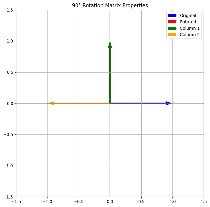 Vector Under Multiple Rotations ```python def show_multiple_rotations(): angles = [0, 45, 90, 135, 180] v = np.array([1, 0]) plt.figure(figsize=(8, 8)) plt.axhline(y=0, color='k', linestyle='-', alpha=0.3) plt.axvline(x=0, color='k', linestyle='-', alpha=0.3) for angle in angles: theta = np.radians(angle) R = np.array([ [np.cos(theta), -np.sin(theta)], [np.sin(theta), np.cos(theta)] ]) v_rot = R @ v plt.quiver(0, 0, v_rot[0], v_rot[1], angles='xy', scale_units='xy', scale=1, label=f'{angle}°') plt.grid(True) plt.xlim(-1.5, 1.5) plt.ylim(-1.5, 1.5) plt.legend() plt.title("Vector Under Multiple Rotations") plt.show() show_multiple_rotations() ``` 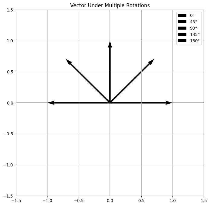 Original basis vectors ```python import numpy as np import matplotlib.pyplot as plt from mpl_toolkits.mplot3d import Axes3D def plot_3d_rotation(axis='z', angle=90): fig = plt.figure(figsize=(10, 10)) ax = fig.add_subplot(111, projection='3d') # Original basis vectors x = np.array([1, 0, 0]) # red y = np.array([0, 1, 0]) # green z = np.array([0, 0, 1]) # blue # Create rotation matrix theta = np.radians(angle) if axis == 'x': R = np.array([ [1, 0, 0], [0, np.cos(theta), -np.sin(theta)], [0, np.sin(theta), np.cos(theta)] ]) elif axis == 'y': R = np.array([ [np.cos(theta), 0, np.sin(theta)], [0, 1, 0], [-np.sin(theta), 0, np.cos(theta)] ]) else: # z-axis R = np.array([ [np.cos(theta), -np.sin(theta), 0], [np.sin(theta), np.cos(theta), 0], [0, 0, 1] ]) # Rotate vectors x_rot = R @ x y_rot = R @ y z_rot = R @ z # Plot original vectors ax.quiver(0, 0, 0, x[0], x[1], x[2], color='r', alpha=0.5, label='Original X') ax.quiver(0, 0, 0, y[0], y[1], y[2], color='g', alpha=0.5, label='Original Y') ax.quiver(0, 0, 0, z[0], z[1], z[2], color='b', alpha=0.5, label='Original Z') # Plot rotated vectors ax.quiver(0, 0, 0, x_rot[0], x_rot[1], x_rot[2], color='darkred', label='Rotated X') ax.quiver(0, 0, 0, y_rot[0], y_rot[1], y_rot[2], color='darkgreen', label='Rotated Y') ax.quiver(0, 0, 0, z_rot[0], z_rot[1], z_rot[2], color='darkblue', label='Rotated Z') # Add axis of rotation if axis == 'x': ax.plot([-1.5, 1.5], [0, 0], [0, 0], 'k--', label='Rotation Axis (X)') elif axis == 'y': ax.plot([0, 0], [-1.5, 1.5], [0, 0], 'k--', label='Rotation Axis (Y)') else: ax.plot([0, 0], [0, 0], [-1.5, 1.5], 'k--', label='Rotation Axis (Z)') ax.set_xlabel('X') ax.set_ylabel('Y') ax.set_zlabel('Z') ax.set_title(f'Rotation around {axis.upper()}-axis by {angle}°') # Set consistent scale ax.set_xlim([-1.5, 1.5]) ax.set_ylim([-1.5, 1.5]) ax.set_zlim([-1.5, 1.5]) plt.legend() plt.show() # Show rotations around each axis for axis in ['x', 'y', 'z']: plot_3d_rotation(axis=axis) ``` 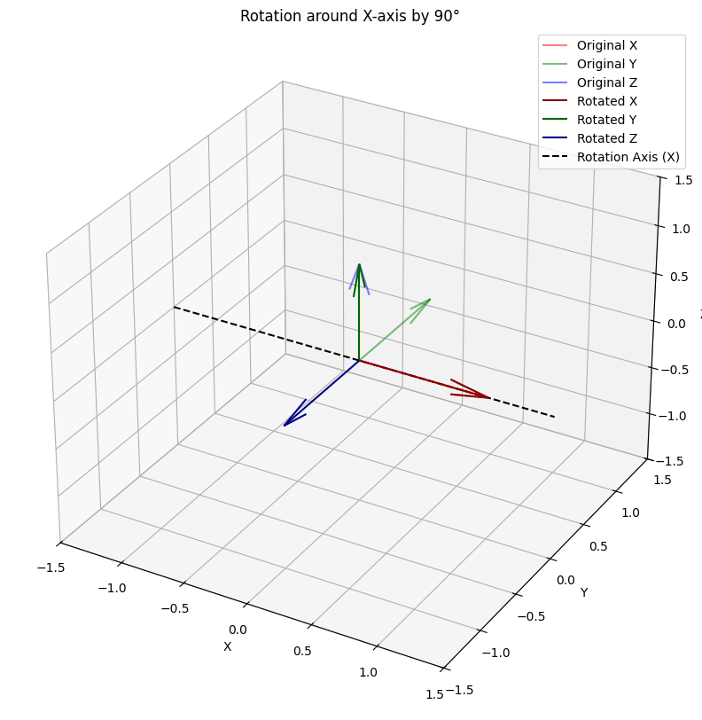 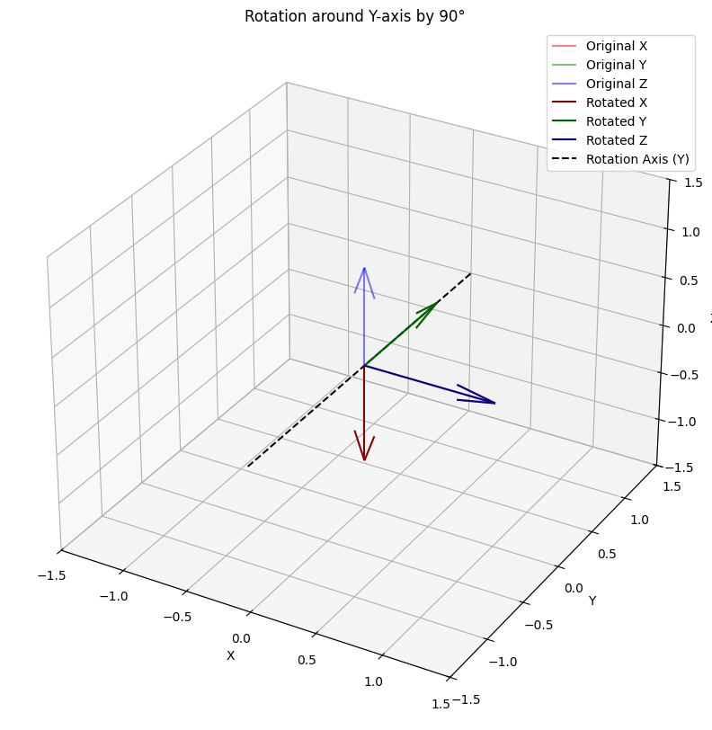  For any 3D rotation matrix R: 1. All columns are perpendicular to each other 2. Each column has length 1 3. R * R^T = Identity matrix Get columns Example with Z-axis rotation ``` Verifying Z-axis rotation matrix: Dot products (should be 0): col1 · col2 = 0.0000000000 col2 · col3 = 0.0000000000 col3 · col1 = 0.0000000000 Column lengths (should be 1): ||col1|| = 1.0000000000 ||col2|| = 1.0000000000 ||col3|| = 1.0000000000 ``` ### What is an orthogonal matrix? Some properties: 1. All the columns are pair-wise orthogonal, so their dot products should be 0. 2. Each column @ itself is 1. 3. All columns norm (geometric length) to 1. Written together, for a square matrix, $\mathbf{Q}^\top\mathbf{Q}=\mathbf{I}$, which is why the inverse equals the transpose. ### An identity matrix is an orthogonal matrix. ```python A = np.identity(3) A ``` ``` array([[1., 0., 0.], [0., 1., 0.], [0., 0., 1.]]) ``` ```python print( A[0]@A[0] ) print( A[0]@A[1] ) print( A[0]@A[2] ) ``` ``` 1.0 0.0 0.0 ``` ### A pure rotation matrix is also orthogonal ```python θ = 20 T = np.array( [ [ np.cos(θ), np.sin(θ) ], [ -np.sin(θ), np.cos(θ) ] ]) T ``` ``` array([[ 0.40808206, 0.91294525], [-0.91294525, 0.40808206]]) ``` ```python np.linalg.norm(T[1]) ``` ``` 1.0 ``` within rounding errors on the 10^-15th order ``` 0.0 ``` ## The Gram-Schmidt procedure to transform a non-orthogonal matrix to an orthogonal one. Gram-Schmidt builds an orthogonal set one vector at a time. Keep the first vector. From each next vector, subtract its projection onto the ones already kept. That projection is the scalar from [Vectors](vectors.html#orthogonal-vector-projection), $\beta=(\mathbf{a}^\top\mathbf{b})/(\mathbf{a}^\top\mathbf{a})$, times the vector it projects onto. What remains is perpendicular to the ones already kept. Below, a random 3 by 3 matrix is tested, and then $\beta$ is computed for $\mathbf{a}=[2,3]$ and $\mathbf{b}=[2,1]$, the same pair as that projection picture. ```python A = np.random.rand(3,3) A ``` ``` array([[0.5499082 , 0.86189965, 0.44453349], [0.54395812, 0.04501642, 0.97553863], [0.49977168, 0.35489466, 0.08201685]]) ``` orthogonality test ``` 1.2428800593764227 0.7715862615401271 1.1148453073751634 ``` a = np.array([2, 3]) b = np.array([2, 1]) beta = np.dot(a,b)/np.dot(a,a) # the orthogonal projection from the head of b, to a projected_beta = a*beta ``` array([0.5499082 , 0.86189965, 0.44453349]) ``` Next: [Calculus](calculus.html).