Neural nets A simple net, its gradient, and the loss surface. math · networks Study sequence: [Vectors](vectors.html) · [Matrices](matrices.html) · [Matrix applications](matrix-applications.html) · [Calculus](calculus.html) · [Big O](big-o.html) · [Geometry](geometry.html) · [Signals](signals.html) · Neural nets · [Distributions](distributions.html) a simple neural net Simple neural network with one hidden layer Loss function: L = (y - ŷ)² ŷ = w2 * sigmoid(w1 * x + b1) + b2 where sigmoid(z) = 1/(1 + e^(-z)) $$\mathcal{L}=(y-\hat{y})^2$$ $$\hat{y}=w_2\,\sigma(w_1 x+b_1)+b_2$$ $$\sigma(z)=\frac{1}{1+e^{-z}}$$ The loss is the square of the miss, how far the prediction $\hat{y}$ is from the target $y$. The prediction is a linear layer, a weighted input plus a bias, passed through the sigmoid, then a second linear layer. A bias is a number added after the weighting, a shift. The sigmoid is the same curve as in [Calculus](calculus.html). $e$ is about 2.718. Example computation for a single data point Forward pass Loss Forward pass ``` 1.1 = 0.5 * 2.0 + 0.1 0.7502601055951177 = sigmoid(1.1) 0.6002080844760942 = 0.8 * 0.7502601055951177 + 0.0 0.15983357571827383 = (1.0 - 0.6002080844760942**2 ``` ## By hand: layer then activation @ alan yeh. ai by hand [https://aibyhand.substack.com/](https://aibyhand.substack.com/) The linear layer, worked by hand, is in [Matrices](matrices.html#by-hand-linear-layer). [https://aibyhand.substack.com/p/w4-activation](https://aibyhand.substack.com/p/w4-activation) ```python def relu(x): return np.where(x >= 0, x, x==0) def sig3(x): cond1 = x >= 2 cond2 = (-1 <= x) & (x <= 1) cond3 = (x <= -2) vals = [1, 0.5, 0] return np.select([cond1, cond2, cond3], vals) def sig5(x): cond1 = x >= 2 cond2 = (1 <= x) & (x < 2) cond3 = (0 <= x) & (x < 1) cond4 = (-2 < x) & (x < 0) cond5 = (x <= -2) vals = [1, 0.7, 0.5, 0.3, 0] return np.select([cond1, cond2, cond3, cond4, cond5], vals) def tanh3(x): cond1 = x >= 2 cond2 = (-1 <= x) & (x <= 1) cond3 = (x <= -2) vals = [1, 0, -1] return np.select([cond1, cond2, cond3], vals) def tanh5(x): cond1 = x >= 2 cond2 = (1 <= x) & (x < 2) cond3 = (0 <= x) & (x < 1) cond4 = (-2 < x) & (x < 0) cond5 = (x <= -2) vals = [1, 0.8, 0, -0.8, -1] return np.select([cond1, cond2, cond3, cond4, cond5], vals) ``` ```python x = L(M([1,-1,0],[1,-2,0],[1,-3,0]), M([3],[2])) relu(x) ``` ``` [[ 1] [-1] [-3]] array([[1], [0], [0]]) ``` ```python x = L(M([1,1,-2],[1,1,-4],[1,1,-6]), M([3],[2])) relu(x) ``` ``` array([[3], [1], [0]]) ``` ```python sig3(L(M([1,-1,0],[1,-2,0],[1,-3,0]), M([3],[2]))) ``` ``` array([[0.5], [0.5], [0. ]]) ``` ```python sig3(L(M([1,-1,3],[1,-2,3],[1,-3,3]), M([3],[2]))) ``` ``` array([[1. ], [1. ], [0.5]]) ``` ```python sig3(L(M([1,-1,-2],[1,-2,-2],[1,-3,-2]), M([3],[2]))) ``` ``` array([[0.5], [0. ], [0. ]]) ``` ```python tanh3(L(M([1,-1,0],[1,-2,0],[1,-3,0]), M([3],[2]))) ``` ``` array([[ 0], [ 0], [-1]]) ``` ```python tanh3(L(M([1,-1,3],[1,-2,3],[1,-3,3]), M([3],[2]))) ``` ``` array([[1], [1], [0]]) ``` ```python tanh3(L(M([1,-1,-2],[1,-2,-2],[1,-3,-2]), M([3],[2]))) ``` ``` array([[ 0], [-1], [-1]]) ``` ```python sig5(L(M([1,1,-2],[1,1,-4],[1,1,-6]), M([3],[2]))) ``` ``` array([[1. ], [0.7], [0.3]]) ``` ```python tanh5(L(M([1,1,-2],[1,1,-4],[1,1,-6]), M([3],[2]))) ``` ``` array([[ 1. ], [ 0.8], [-0.8]]) ``` ```python sig5(L(M([1,0,0],[0,1,0],[1,1,0],[-1,-1,0],[1,-1,0],[-1,1,0],[-1,0,0],[0,-1,0],[0,0,0]), M([3],[2]))) ``` ``` array([[1. ], [1. ], [1. ], [0. ], [0.7], [0.3], [0. ], [0. ], [0.5]]) ``` ```python tanh5(L(M([1,0,0],[0,1,0],[1,1,0],[-1,-1,0],[1,-1,0],[-1,1,0],[-1,0,0],[0,-1,0],[0,0,0]), M([3],[2]))) ``` ``` array([[ 1. ], [ 1. ], [ 1. ], [-1. ], [ 0.8], [-0.8], [-1. ], [-1. ], [ 0. ]]) ``` ```python L(M([1,1,-5]), M([3],[1])) ``` ``` array([[-1]]) ``` ```python relu(L(M([1,-1,0]), M([3],[1]))) ``` ``` array([[2]]) ``` ```python x = L(M([2,1,1]), M([2],[-1])) print(x) relu(x) ``` ``` [[4]] array([[4]]) ``` ```python x = L(M([2,1,-5]), M([2],[-1])) print(x) relu(x) ``` ``` [[-2]] array([[0]]) ``` ```python sig3(L(M([1,-1,-1]), M([4],[2]))) ``` ``` array([[0.5]]) ``` ```python sig3(L(M([2,-1,0]), M([3],[4]))) ``` ``` array([[1.]]) ``` ```python x = L(M([1,0,1,-2]), M([2],[5],[1])) print(x) relu(x) ``` ``` [[1]] array([[1]]) ``` ```python x = L(M([1,-1,0,2]), M([2],[5],[1])) print(x) relu(x) ``` ``` [[-1]] array([[0]]) ``` ```python x = L(M([1,-1,0,2]), M([2],[5],[1])) print(x) sig3(x) ``` ``` [[-1]] array([[0.5]]) ``` ```python x = L(M([0,1,-1],[1,0,0],[1,0,-1]), M([4],[6])) print(x) relu(x) ``` ``` [[5] [4] [3]] array([[5], [4], [3]]) ``` ```python x = L(M([1,1,-2],[1,-1,-2],[0,-1,-2]), M([5],[2])) print(x) relu(x) ``` ``` [[ 5] [ 1] [-4]] array([[5], [1], [0]]) ``` ```python x = L(M([1,-1,0],[1,-2,0],[1,-3,0]), M([3],[2])) print(x) relu(x) ``` ``` [[ 1] [-1] [-3]] array([[1], [0], [0]]) ``` ```python x = L(M([1,1,1,0],[1,1,0,0],[1,0,0,0]), M([3],[1],[2])) print(x) relu(x) ``` ``` [[6] [4] [3]] array([[6], [4], [3]]) ``` ```python x = L(M([1,1,0,0],[1,0,-1,0],[1,-1,0,0]), M([2],[3],[4])) print(x) relu(x) ``` ``` [[ 5] [-2] [-1]] array([[5], [0], [0]]) ``` ```python x = L(M([0,1,0,-3],[1,0,-1,0],[1,-1,0,0]), M([5],[2],[-3])) print(x) relu(x) ``` ``` [[-1] [ 8] [ 3]] array([[0], [8], [3]]) ``` ```python relu(L(M([1,1,0]), M([3],[2]))) ``` ``` array([[5]]) ``` ```python relu(L(M([1,-1,0]), M([4],[5]))) ``` ``` array([[0]]) ``` ```python relu(L(M([-1,1,0]), M([3],[5]))) ``` ``` array([[2]]) ``` ```python relu(L(M([1,-2,0]), M([3],[2]))) ``` ``` array([[0]]) ``` ```python relu(L(M([1,-1,-2]), M([3],[2]))) ``` ``` array([[0]]) ``` ```python relu(L(M([1,1,1,0]), M([-4],[2],[3]))) ``` ``` array([[1]]) ``` ```python relu(L(M([1,-1,1,0]), M([2],[3],[1]))) ``` ``` array([[0]]) ``` ```python relu(L(M([1,1,-2,0]), M([4],[1],[3]))) ``` ``` array([[0]]) ``` ```python relu(L(M([1,-1,0,0],[1,0,-1,0],[1,0,0,0]), M([2],[4],[3]))) ``` ``` array([[0], [0], [2]]) ``` ```python sig3(L(M([1,-1,0,0],[1,0,-1,0],[1,0,0,0]), M([2],[4],[3]))) ``` ``` array([[0. ], [0.5], [1. ]]) ``` # gradients A partial derivative is the slope of a function when you move only one input and hold the others still. The gradient is every partial derivative gathered into one vector. It points toward the steepest increase. The surface below is $F(i,j)=i/(j+3)$. Moving only $i$, the slope is $1/(j+3)$. Moving only $j$, the slope is $-i/(j+3)^2$. Those two slopes are the gradient of $F$. Original discrete version: ```python # Original discrete version: f = [0, 1, 2] x = [3, 4, 5] # To make it continuous, we can observe that: # - i represents the row number (from f) # - j represents the column number (from x) # The pattern is: F(i,j) = i/(j+3) # As a continuous function: def F(i, j): return i/(j+3) # Now we can find any point, even non-integer values: # F(1.5, 0.5) would be valid # F(π, 2) would be valid # This represents how F changes as we move vertically def dF_di(i, j): return 1/(j+3) # derivative of i/(j+3) with respect to i # This represents how F changes as we move horizontally def dF_dj(i, j): return -i/(j+3)**2 # derivative of i/(j+3) with respect to j import numpy as np import matplotlib.pyplot as plt from mpl_toolkits.mplot3d import Axes3D # Example plotting code: i = np.linspace(0, 2, 100) j = np.linspace(0, 2, 100) I, J = np.meshgrid(i, j) Z = I/(J+3) fig = plt.figure(figsize=(10,10)) ax = fig.add_subplot(111, projection='3d') ax.plot_surface(I, J, Z, cmap='turbo') ax.view_init(elev=20, azim=75) plt.show() ``` 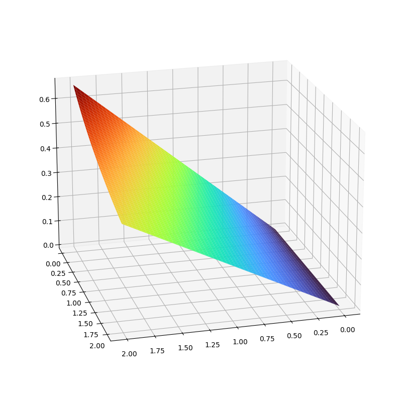 hessian loss matrix The Hessian is the matrix of second derivatives: the derivative of the gradient, which records how the slope itself bends. A second derivative is the slope of the slope. The picture is a surface built from that bending. The wider landscape below is the same kind of surface drawn over a larger window. ```python # hessian loss matrix import numpy as np import matplotlib.pyplot as plt from mpl_toolkits.mplot3d import Axes3D from matplotlib.widgets import Slider # Create a function that generates a random Hessian-like surface def generate_hessian_surface(n_points, input_dim): # Create random weights to simulate network parameters weights = np.random.randn(input_dim) # Create grid of points x = np.linspace(-2, 2, n_points) y = np.linspace(-2, 2, n_points) X, Y = np.meshgrid(x, y) # Simulate loss surface with quadratic form (Hessian approximation) Z = np.zeros_like(X) for i in range(input_dim): Z += weights[i] * (X**2 + Y**2) / (i + 1) # Add some noise to make it more realistic Z += np.random.randn(n_points, n_points) * 0.1 return X, Y, Z # Create the figure and 3D plot fig = plt.figure(figsize=(12, 8)) ax = fig.add_subplot(111, projection='3d') # Initial plot n_points = 50 initial_dim = 5 X, Y, Z = generate_hessian_surface(n_points, initial_dim) surface = ax.plot_surface(X, Y, Z, cmap='viridis') # Add colorbar fig.colorbar(surface, ax=ax, label='Loss Value') # Labels ax.set_xlabel('Parameter 1') ax.set_ylabel('Parameter 2') ax.set_zlabel('Loss') ax.set_title(f'Loss Landscape with {initial_dim} Input Dimensions') # Add slider for input dimensions ax_slider = plt.axes([0.1, 0.02, 0.65, 0.03]) slider = Slider( ax=ax_slider, label='Input Dimensions', valmin=1, valmax=20, valinit=initial_dim, valstep=1 ) # Update function for slider def update(val): ax.clear() X, Y, Z = generate_hessian_surface(n_points, int(val)) surface = ax.plot_surface(X, Y, Z, cmap='viridis') ax.set_xlabel('Parameter 1') ax.set_ylabel('Parameter 2') ax.set_zlabel('Loss') ax.set_title(f'Loss Landscape with {int(val)} Input Dimensions') fig.canvas.draw_idle() slider.on_changed(update) # Add rotation controls def rotate_view(event): if event.key == 'left': ax.view_init(elev=ax.elev, azim=ax.azim - 10) elif event.key == 'right': ax.view_init(elev=ax.elev, azim=ax.azim + 10) elif event.key == 'up': ax.view_init(elev=ax.elev + 10, azim=ax.azim) elif event.key == 'down': ax.view_init(elev=ax.elev - 10, azim=ax.azim) fig.canvas.draw() fig.canvas.mpl_connect('key_press_event', rotate_view) # Add some interactivity instructions plt.figtext(0.02, 0.95, 'Use arrow keys to rotate view', fontsize=9) plt.show() ``` 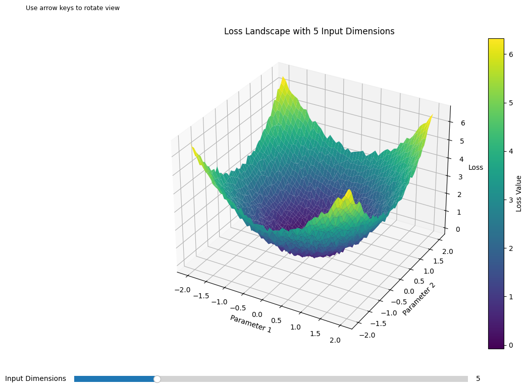 a wider loss landscape ```python # a wider loss landscape import numpy as np import matplotlib.pyplot as plt from mpl_toolkits.mplot3d import Axes3D import matplotlib.animation as animation from matplotlib.widgets import Slider, Button # Create more interesting Hessian-like surface def generate_dynamic_surface(n_points, time, complexity): x = np.linspace(-2, 2, n_points) y = np.linspace(-2, 2, n_points) X, Y = np.meshgrid(x, y) # Base quadratic surface Z = 0.5 * (X**2 + Y**2) # Add time-varying components Z += 0.5 * np.sin(complexity * X + time) * np.cos(complexity * Y + time) Z += 0.3 * np.cos(complexity * X - time) * np.sin(complexity * Y - time) # Add moving wave patterns Z += 0.2 * np.sin(np.sqrt(X**2 + Y**2) - time) # Add some randomness that changes with time np.random.seed(int(time * 100)) Z += np.random.randn(n_points, n_points) * 0.1 return X, Y, Z # Alternative surface generation for different behaviors def generate_alternative_surface(n_points, time, complexity): x = np.linspace(-2, 2, n_points) y = np.linspace(-2, 2, n_points) X, Y = np.meshgrid(x, y) # Create spiral patterns R = np.sqrt(X**2 + Y**2) theta = np.arctan2(Y, X) Z = np.sin(R - time) * np.cos(theta * complexity) Z += 0.5 * (X**2 + Y**2) * np.sin(time) return X, Y, Z # Set up the figure and 3D plot fig = plt.figure(figsize=(12, 8)) ax = fig.add_subplot(111, projection='3d') # Initial parameters n_points = 50 complexity = 2 time = 0 # Create initial surface X, Y, Z = generate_dynamic_surface(n_points, time, complexity) surface = ax.plot_surface(X, Y, Z, cmap='viridis') # Add colorbar fig.colorbar(surface, ax=ax, label='Loss Value') # Labels ax.set_xlabel('Parameter 1') ax.set_ylabel('Parameter 2') ax.set_zlabel('Loss') ax.set_title('Dynamic Loss Landscape') # Animation speed control speed = 1.0 # Add sliders ax_complexity = plt.axes([0.1, 0.02, 0.65, 0.03]) ax_speed = plt.axes([0.1, 0.06, 0.65, 0.03]) s_complexity = Slider( ax=ax_complexity, label='Complexity', valmin=0.1, valmax=5.0, valinit=complexity ) s_speed = Slider( ax=ax_speed, label='Speed', valmin=0.1, valmax=3.0, valinit=speed ) # Animation update function def update(frame): ax.clear() # Get current complexity and speed values current_complexity = s_complexity.val current_time = frame * s_speed.val # Generate new surface X, Y, Z = generate_dynamic_surface(n_points, current_time, current_complexity) # Plot new surface surface = ax.plot_surface(X, Y, Z, cmap='viridis') # Set labels and limits ax.set_xlabel('Parameter 1') ax.set_ylabel('Parameter 2') ax.set_zlabel('Loss') ax.set_title(f'Dynamic Loss Landscape (t={current_time:.1f})') # Set consistent view limits ax.set_zlim(-2, 4) # Set viewing angle ax.view_init(elev=30, azim=frame/2) # Slowly rotate view return surface, # Create animation anim = animation.FuncAnimation( fig, update, frames=200, interval=50, blit=False, repeat=True ) # Add pause/play button ax_button = plt.axes([0.8, 0.02, 0.1, 0.04]) btn = Button(ax_button, 'Pause/Play') # Pause/play functionality anim_running = True def onClick(event): global anim_running if anim_running: anim.event_source.stop() anim_running = False else: anim.event_source.start() anim_running = True btn.on_clicked(onClick) # Add rotation controls def rotate_view(event): if event.key == 'left': ax.view_init(elev=ax.elev, azim=ax.azim - 10) elif event.key == 'right': ax.view_init(elev=ax.elev, azim=ax.azim + 10) elif event.key == 'up': ax.view_init(elev=ax.elev + 10, azim=ax.azim) elif event.key == 'down': ax.view_init(elev=ax.elev - 10, azim=ax.azim) fig.canvas.mpl_connect('key_press_event', rotate_view) # Add instructions plt.figtext(0.02, 0.95, 'Use arrow keys to adjust view\nUse sliders to control complexity and speed', fontsize=9) plt.show() ``` 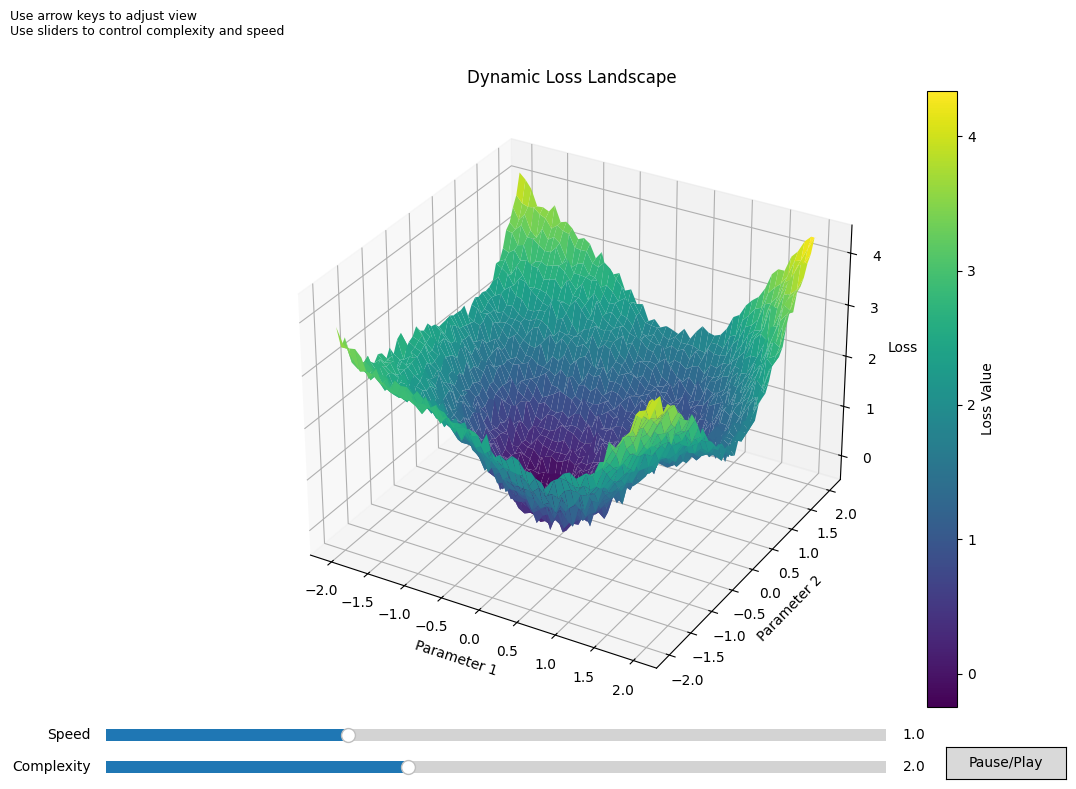 Next: [Distributions](distributions.html).