Signals Frequency modulated waves, chirps, and a sampled sine. math · signals Study sequence: [Vectors](vectors.html) · [Matrices](matrices.html) · [Matrix applications](matrix-applications.html) · [Calculus](calculus.html) · [Big O](big-o.html) · [Geometry](geometry.html) · Signals · [Neural nets](neural-nets.html) · [Distributions](distributions.html) Frequency Modulated Waveform Frequency modulation means the pitch of the wave is itself changing. The carrier is the fast wave, here 100 Hz. A hertz is one cycle per second. The modulating wave is the slow wave, here 2 Hz, and it is added inside the phase, the position inside the cycle: $$s(t)=\sin\left(2\pi f_c t+\beta\sin(2\pi f_m t)\right)$$ with $f_c=100$, $f_m=2$, and $\beta=2$, the modulation index in the code. ```python import numpy as np import matplotlib.pyplot as plt # Define parameters carrier_freq = 100.0 # Carrier frequency in Hz modulating_freq = 2.0 # Modulating frequency in Hz mod_index = 2.0 # Modulation index sample_rate = 10000 # Samples per second duration = 1.0 # Duration in seconds # Create time array t = np.linspace(0, duration, int(sample_rate * duration), endpoint=False) # Generate modulating signal modulating_signal = np.sin(2 * np.pi * modulating_freq * t) # Generate frequency modulated signal fm_signal = np.sin(2 * np.pi * carrier_freq * t + mod_index * modulating_signal) # Plot the FM waveform plt.figure(figsize=(10, 4)) plt.plot(t, fm_signal) plt.title("Frequency Modulated Waveform") plt.xlabel("Time (s)") plt.ylabel("Amplitude") plt.grid(True) plt.show() ``` 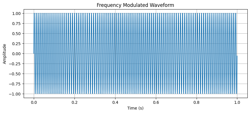 FM Chirp A chirp is a wave whose frequency slides. This one is $$\sin\left(2\pi\left(f_0 t+\frac{1}{2} k t^2\right)\right)$$ with $f_0$ the start frequency and $k=(f_1-f_0)/\text{duration}$ the rate of the slide. ```python start_freq = 100.0 end_freq = 500.0 k = (end_freq - start_freq) / duration chirp_signal = np.sin(2 * np.pi * (start_freq * t + 0.5 * k * t**2)) plt.figure(figsize=(10, 4)) plt.plot(t, chirp_signal) plt.title("FM Chirp") plt.xlabel("Time (s)") plt.ylabel("Amplitude") plt.grid(True) plt.show() ``` 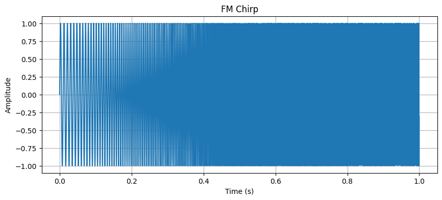 Bandwidth of the Linear FM Chirp (100 Hz to 500 Hz) The instantaneous frequency is the pitch at time $t$. For this linear chirp it is the straight line $$f(t)=f_0+kt$$ from 100 Hz to 500 Hz. The bandwidth is the width of that span, $500-100=400$ Hz. Bandwidth is how wide a band of pitches the signal occupies. ```python bandwidth = end_freq - start_freq inst_freq = start_freq + k * t plt.figure(figsize=(10, 4)) plt.plot(t, inst_freq, label="Instantaneous Frequency") plt.title(f"Bandwidth of the Linear FM Chirp ({start_freq} Hz to {end_freq} Hz)") plt.xlabel("Time (s)") plt.ylabel("Frequency (Hz)") plt.grid(True) plt.legend() plt.show() ``` 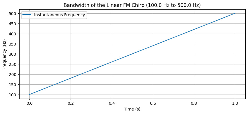 Magnitude Spectrum of FM Chirp A Fourier transform splits a wave into pure tones, one sine at each pitch. The magnitude is how much of each pitch is present. The code takes the absolute value of the fast Fourier transform, the FFT, which is that split for a list of samples. A sample is one recorded height at one instant. ```python # Compute FFT of chirp signal fft_chirp = np.fft.fft(chirp_signal) freq = np.fft.fftfreq(len(t), t[1] - t[0]) # Plot magnitude spectrum plt.figure(figsize=(10, 4)) plt.plot(freq[:1000], np.abs(fft_chirp)[:1000]) plt.title("Magnitude Spectrum of FM Chirp") plt.xlabel("Frequency (Hz)") plt.ylabel("Magnitude") plt.grid(True) plt.show() ``` 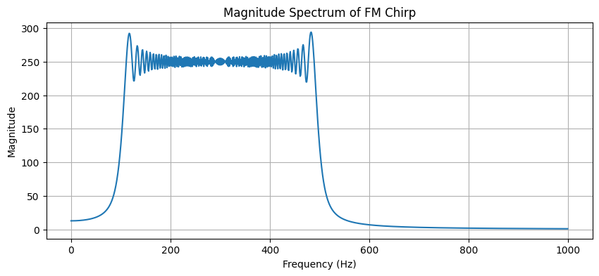 Generate chirp De-chirping, called range compression in the figure, takes the Fourier transform of the chirp. A delay, a shift in time, moves where the compressed peak sits. ```python import numpy as np import matplotlib.pyplot as plt # Create a chirp signal def create_chirp(t, f0, f1, t1): return np.exp(1j * 2 * np.pi * (f0 * t + ((f1-f0)/(2*t1)) * t**2)) # Parameters duration = 1000 # samples t = np.linspace(0, 1, duration) f0 = 0 # start frequency f1 = 100 # end frequency # Generate chirp chirp = create_chirp(t, f0, f1, 1) # Perform de-chirping (range compression) dechirped = np.fft.fftshift(np.fft.fft(chirp)) # Create subplot fig, (ax1, ax2) = plt.subplots(2, 1, figsize=(12, 8)) # Plot original chirp ax1.plot(t, np.real(chirp)) ax1.set_title('Original Chirp Signal') ax1.set_xlabel('Time') ax1.set_ylabel('Amplitude') ax1.grid(True) # Plot de-chirped signal ax2.plot(np.abs(dechirped)) ax2.set_title('After De-chirping (Range Compressed)') ax2.set_xlabel('Frequency') ax2.set_ylabel('Magnitude') ax2.grid(True) plt.tight_layout() plt.show() ``` 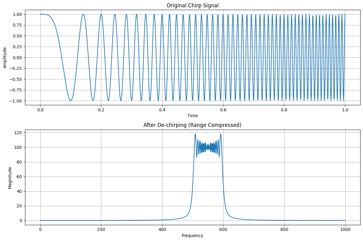 Create multiple chirps with different delays Each delay is a copy of the chirp shifted in time. After the same transform, each delay becomes its own peak. ```python import numpy as np import matplotlib.pyplot as plt # Create multiple chirps with different delays def create_delayed_chirps(t, f0, f1, t1, delays, amplitudes): signal = np.zeros_like(t, dtype=complex) for delay, amp in zip(delays, amplitudes): # Shift the chirp by delay and multiply by amplitude shifted_t = t - delay signal += amp * np.exp(1j * 2 * np.pi * (f0 * shifted_t + ((f1-f0)/(2*t1)) * shifted_t**2)) * (shifted_t >= 0) return signal # Parameters duration = 1000 t = np.linspace(0, 1, duration) f0 = 0 f1 = 100 # Create three targets at different ranges with different amplitudes delays = [0.2, 0.4, 0.6] # Different time delays amplitudes = [1.0, 0.7, 0.5] # Different reflection strengths # Generate combined signal combined_chirps = create_delayed_chirps(t, f0, f1, 1, delays, amplitudes) # Perform de-chirping dechirped = np.fft.fftshift(np.fft.fft(combined_chirps)) # Create subplot fig, (ax1, ax2) = plt.subplots(2, 1, figsize=(12, 8)) # Plot original signal ax1.plot(t, np.real(combined_chirps)) ax1.set_title('Original Signal with Multiple Chirps') ax1.set_xlabel('Time') ax1.set_ylabel('Amplitude') ax1.grid(True) # Plot de-chirped signal ax2.plot(np.abs(dechirped)) ax2.set_title('After De-chirping: Multiple Peaks') ax2.set_xlabel('Range Bin') ax2.set_ylabel('Magnitude') ax2.grid(True) plt.tight_layout() plt.show() ``` 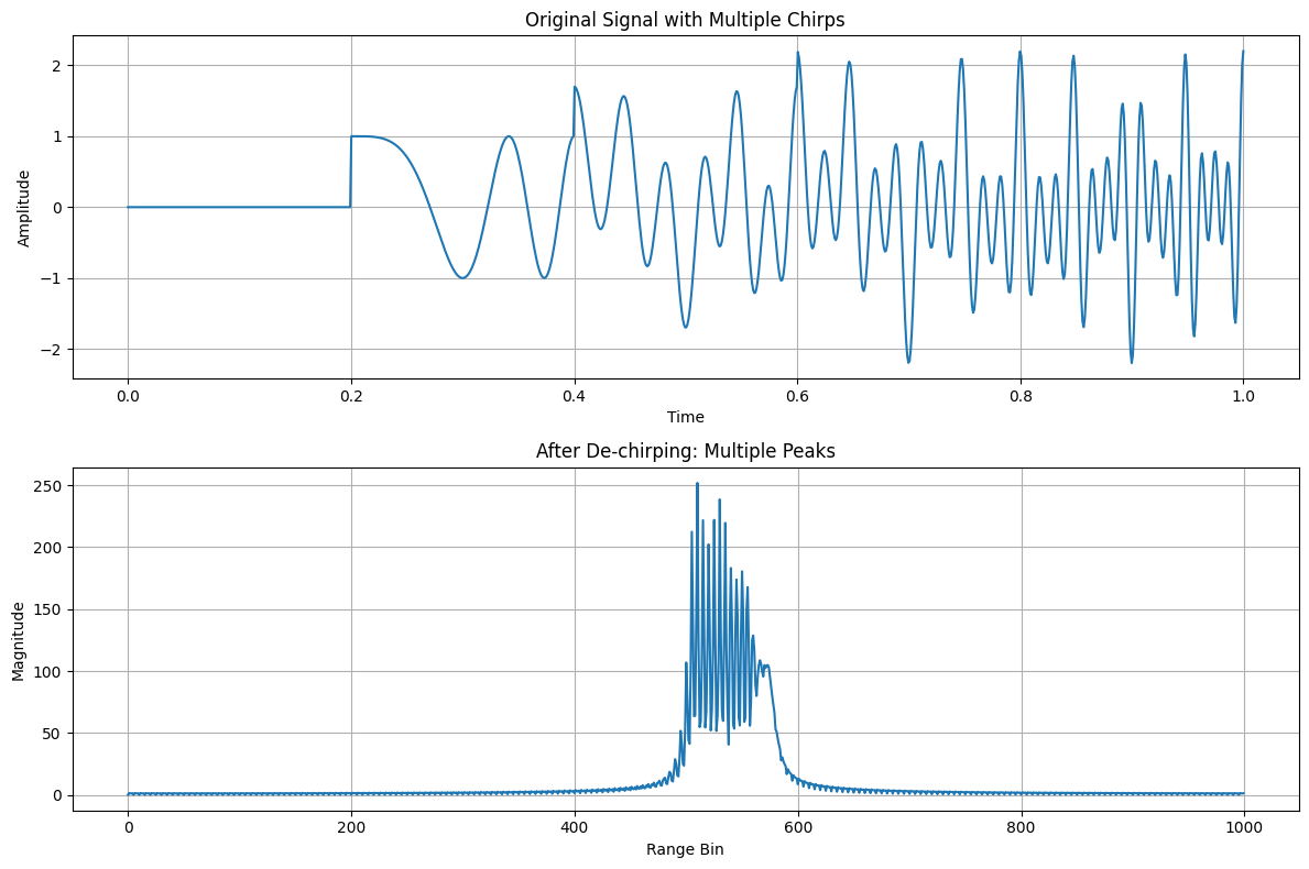 Visualizing an FM Linear Chirp Being Emitted, Received, Range Compressed, This chirp is the complex form of the same slide, $$\exp\left(i\,2\pi\left(f_0 t+\frac{f_1-f_0}{2 t_1}t^2\right)\right)$$ with $f_0=30$ and $f_1=200$ in the code's own units. A complex exponential $e^{i\phi}$ is a cosine plus $i$ times a sine, so the plot can draw a real part and an imaginary part of the same wave. A scatterer is a reflector. One is placed at range bin 300, and each later pulse is multiplied by an extra phase, the Doppler factor in the code. Doppler here is that extra phase from pulse to pulse. Range compression is a Fourier transform along each pulse. Azimuth compression is a Fourier transform across pulses. ```python # Jupyter Notebook Example: # Visualizing an FM Linear Chirp Being Emitted, Received, Range Compressed, # and Azimuth (Doppler) Compressed in Matplotlib # ------------------------------------------------------------------------ # In[1]: import numpy as np import matplotlib.pyplot as plt def create_chirp(t, f0, f1, t1): """ Creates a linear frequency-modulated (FM) chirp signal. t : 1D array of time samples f0 : start frequency f1 : end frequency t1 : total duration (in the same units as t) Returns: A complex 1D numpy array representing the chirp. """ return np.exp(1j * 2 * np.pi * (f0 * t + ((f1 - f0) / (2 * t1)) * t**2)) # In[2]: # 1) Define parameters and create the "emitted" chirp duration = 1000 # Number of range samples (fast time) t = np.linspace(0, 1, duration) f0 = 30 # Start frequency (arbitrary units) f1 = 200 # End frequency (arbitrary units) chirp_emitted = create_chirp(t, f0, f1, 1) # In[3]: # 2) Simulate "received" data in a 2D array (pulses vs. range) # - We'll assume there's a single strong scatterer at a certain range bin # - We'll also add a slight Doppler shift each pulse to simulate motion num_pulses = 64 # Azimuth dimension (slow time) scatterer_range_bin = 300 # Where the scatterer "lives" in the range dimension scatterer_phase_shift = 0.05 # Doppler shift factor per pulse # Initialize the receive array received_data = np.zeros((num_pulses, duration), dtype=complex) for pulse_idx in range(num_pulses): # Slight Doppler phase shift for each pulse doppler_phase = np.exp(1j * 2 * np.pi * scatterer_phase_shift * pulse_idx * t) # Copy chirp, add Doppler shift pulse_signal = chirp_emitted * doppler_phase # Place the scatterer as if the echo returns from that range bin # In reality, you'd convolve with system impulse response, # but here, we'll inject a scaled, shifted version for demonstration. shifted_pulse = np.zeros_like(pulse_signal) if scatterer_range_bin < duration: shifted_pulse[scatterer_range_bin:] = pulse_signal[:duration - scatterer_range_bin] received_data[pulse_idx, :] = shifted_pulse # In[4]: # 3) Range Compression: # - FFT along the "range" dimension (axis=1) on each pulse range_compressed = np.fft.fft(received_data, axis=1) # 4) Doppler (Azimuth) Compression: # - FFT along the azimuth dimension (axis=0) # - fftshift to center zero-Doppler in the middle doppler_compressed = np.fft.fftshift(np.fft.fft(range_compressed, axis=0), axes=0) # In[5]: # Create visualizations for each step in one figure fig, axs = plt.subplots(2, 2, figsize=(14, 10)) # (a) Emitted Chirp (Time Domain) axs[0, 0].plot(t, np.real(chirp_emitted), label='Real Part') axs[0, 0].plot(t, np.imag(chirp_emitted), label='Imag Part', alpha=0.7) axs[0, 0].set_title("1) Emitted Chirp in Time Domain") axs[0, 0].set_xlabel("Time (normalized)") axs[0, 0].set_ylabel("Amplitude") axs[0, 0].grid(True) axs[0, 0].legend() # (b) Received Data (Raw 2D) im1 = axs[0, 1].imshow( np.abs(received_data), aspect='auto', cmap='viridis', extent=[0, duration, 0, num_pulses] ) axs[0, 1].set_title("2) Received Data (Range vs. Pulse)") axs[0, 1].set_xlabel("Range Samples") axs[0, 1].set_ylabel("Pulse Index") fig.colorbar(im1, ax=axs[0, 1], fraction=0.046, pad=0.04) # (c) After Range Compression im2 = axs[1, 0].imshow( np.abs(range_compressed), aspect='auto', cmap='viridis', extent=[0, duration, 0, num_pulses] ) axs[1, 0].set_title("3) Range-Compressed Data") axs[1, 0].set_xlabel("Range Frequency Bins") axs[1, 0].set_ylabel("Pulse Index") fig.colorbar(im2, ax=axs[1, 0], fraction=0.046, pad=0.04) # (d) Final Image: Azimuth/Doppler Compression im3 = axs[1, 1].imshow( np.abs(doppler_compressed), aspect='auto', cmap='viridis', extent=[0, duration, -num_pulses/2, num_pulses/2] ) axs[1, 1].set_title("4) Azimuth Compressed (Range vs. Doppler)") axs[1, 1].set_xlabel("Range Frequency Bins") axs[1, 1].set_ylabel("Doppler Frequency (shifted)") fig.colorbar(im3, ax=axs[1, 1], fraction=0.046, pad=0.04) plt.tight_layout() plt.show() ``` 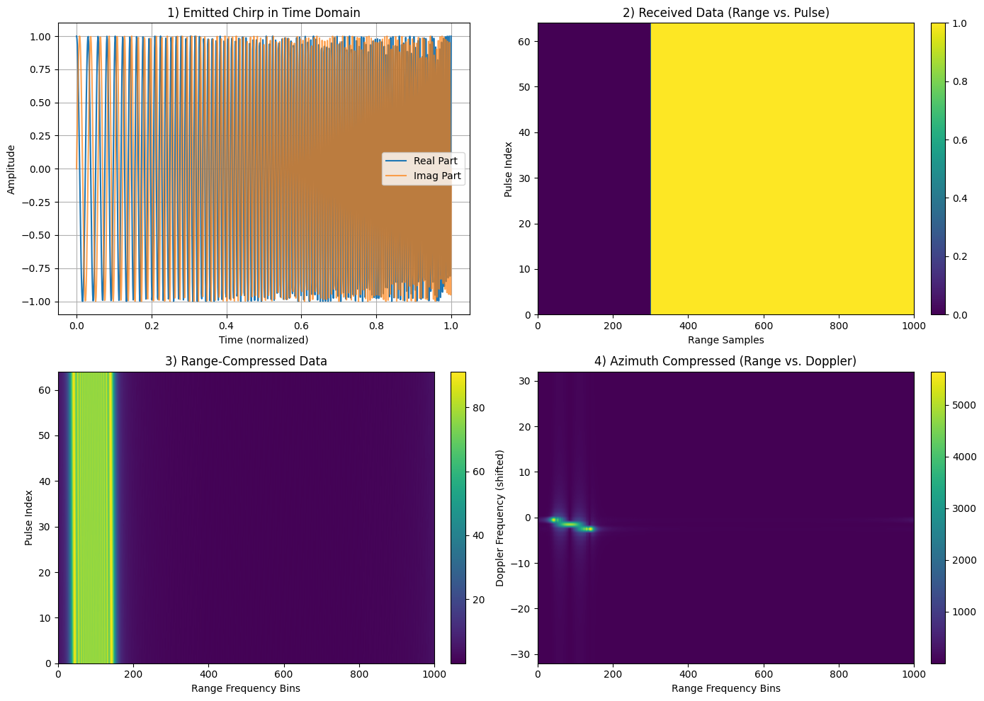 Phase Change vs Two-Way Distance Phase is the position inside one cycle, measured in radians. The code uses a wavelength of 0.03 m, the approximate length of one cycle at this band, and $$\phi=\frac{4\pi d}{\lambda}$$ where $d$ is the two-way distance, out and back, and $\lambda$ is the wavelength. The $4\pi$ is two trips times the $2\pi$ radians in one cycle. Wrapped phase folds that growing angle back into a single cycle by the remainder after division by $2\pi$, which is what `np.mod(phase_change, 2*np.pi)` computes. ```python # Create a new figure for phase change analysis plt.figure(figsize=(14, 6)) # Calculate phase change wavelength = 0.03 # X-band wavelength in meters (approximate) two_way_distance = np.linspace(0, 1000, 1000) # Range of distances in meters phase_change = (4 * np.pi * two_way_distance) / wavelength # 4π because of two-way travel # Plot phase change vs distance plt.subplot(1, 2, 1) plt.plot(two_way_distance, phase_change, 'b-') plt.title('Phase Change vs Two-Way Distance') plt.xlabel('Two-Way Distance (m)') plt.ylabel('Phase Change (radians)') plt.grid(True) # Plot wrapped phase to show cyclic nature plt.subplot(1, 2, 2) plt.plot(two_way_distance, np.mod(phase_change, 2*np.pi), 'r-') plt.title('Wrapped Phase vs Two-Way Distance') plt.xlabel('Two-Way Distance (m)') plt.ylabel('Wrapped Phase (radians)') plt.grid(True) plt.tight_layout() plt.show() ``` 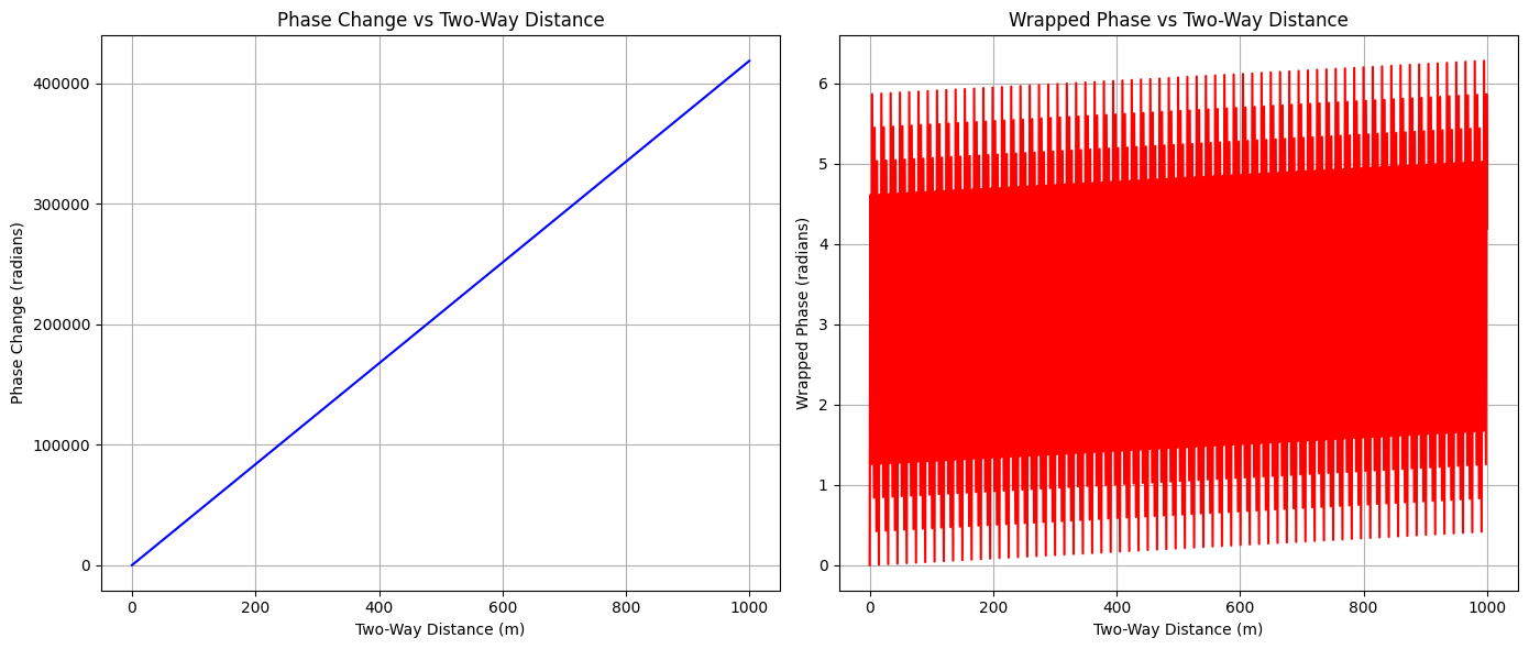 Individual Phase Contributions from Multiple Scatterers Each scatterer contributes a wave whose phase depends on how far it sits from the range being plotted: $$\phi_i=\frac{4\pi (d-d_i)}{\lambda}$$ The drawn contribution is the amplitude times $\cos\phi_i$. Amplitude is the height of that scatterer's wave. The combined signal adds the complex versions, amplitude times $e^{i\phi_i}$. The magnitude of that sum is the strength of the combined wave. ```python # Create a figure to illustrate phase contributions from multiple scatterers plt.figure(figsize=(14, 8)) # Define parameters num_scatterers = 4 distances = np.array([200, 400, 600, 800]) # Distances of scatterers in meters amplitudes = np.array([1.0, 0.8, 0.6, 0.4]) # Relative amplitudes of scatterers two_way_distance = np.linspace(0, 1000, 1000) wavelength = 0.03 # X-band wavelength in meters # Calculate individual phase contributions phase_contributions = np.zeros((num_scatterers, len(two_way_distance))) total_signal = np.zeros(len(two_way_distance), dtype=complex) for i in range(num_scatterers): # Phase contribution from each scatterer phase = (4 * np.pi * (two_way_distance - distances[i])) / wavelength phase_contributions[i] = amplitudes[i] * np.cos(phase) total_signal += amplitudes[i] * np.exp(1j * phase) # Plot individual contributions plt.subplot(2, 1, 1) for i in range(num_scatterers): plt.plot(two_way_distance, phase_contributions[i], label=f'Scatterer at {distances[i]}m') plt.title('Individual Phase Contributions from Multiple Scatterers') plt.xlabel('Range Distance (m)') plt.ylabel('Amplitude') plt.grid(True) plt.legend() # Plot combined signal plt.subplot(2, 1, 2) plt.plot(two_way_distance, np.abs(total_signal), 'k-', label='Combined Magnitude') plt.plot(two_way_distance, np.real(total_signal), 'b--', label='Combined Real Part') plt.title('Combined Signal from All Scatterers') plt.xlabel('Range Distance (m)') plt.ylabel('Amplitude') plt.grid(True) plt.legend() plt.tight_layout() plt.show() ``` 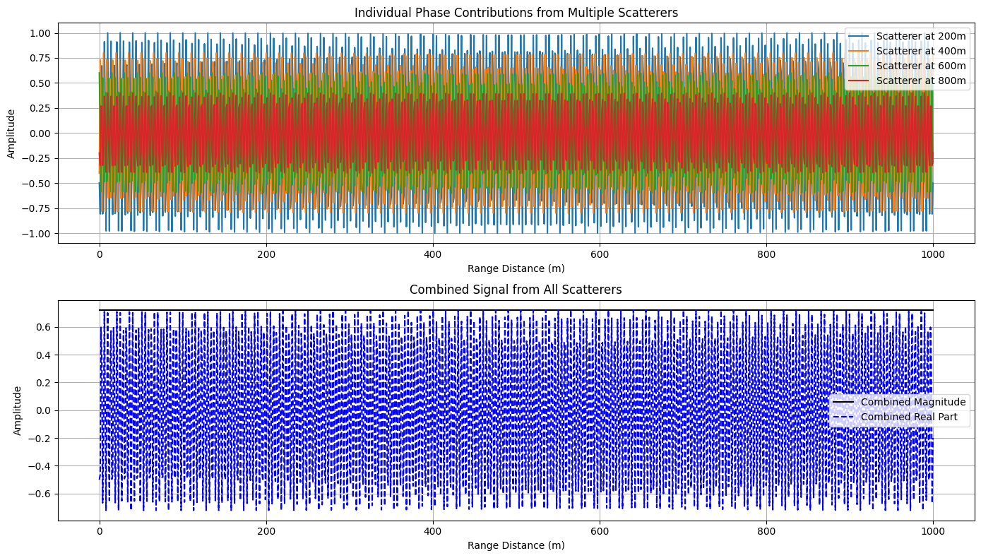 ## Quantization A sine wave of amplitude $A$, frequency $f$, sampled at $f_s$ samples per second, is $$A\sin(2\pi f t)$$ with $A=1$, $f=5$ Hz, and $f_s=44100$. Sampling means recording the height at evenly spaced times. The wave has continuously many heights. Uniform bins cut that range of heights into equal steps. The later plot uses 4 bins, so every sample is replaced by one of four levels. The histogram counts how many samples land in each step. sine wave ```python import numpy as np import matplotlib.pyplot as plt # from scipy.interpolate import interp # Parameters fs = 44100 # Sampling frequency (Hz) T = 1 # Duration of signal (seconds) frequency = 5 # Frequency of sine wave (Hz) amplitude = 1 # Amplitude of sine wave num_samples = fs * T # Total number of samples time = np.linspace(0, T, num_samples, endpoint=False) # Time axis sine_wave = amplitude * np.sin(2 * np.pi * frequency * time) ``` ```python plt.plot(sine_wave) ``` 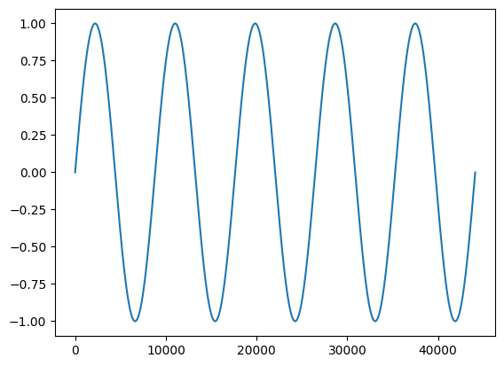 histogram of the sine wave ```python plt.hist(sine_wave, bins=256) plt.show() ``` 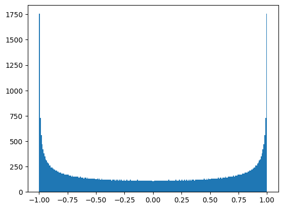 sine wave in 4 uniform bins ```python from sklearn.preprocessing import KBinsDiscretizer ``` ```python n_bins = 4 reshaped_sine_wave = sine_wave.reshape(-1, 1) encoder = KBinsDiscretizer( n_bins=n_bins, encode='ordinal', strategy='uniform', random_state=0, ) compressed_sine_wave = encoder.fit_transform(reshaped_sine_wave) ``` ```python plt.plot(compressed_sine_wave) ``` 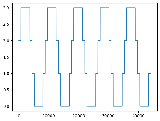 histogram of the binned wave ```python plt.hist(compressed_sine_wave, bins=256) plt.show() ``` 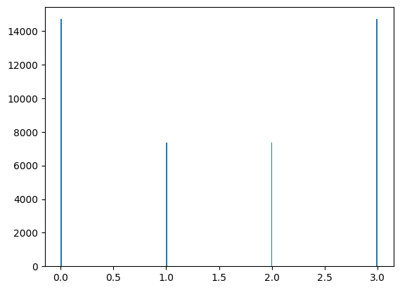 Next: [Neural nets](neural-nets.html).