Vectors Assume all vectors are columnar unless indicated. math · vectors Study sequence: Vectors · [Matrices](matrices.html) · [Matrix applications](matrix-applications.html) · [Calculus](calculus.html) · [Big O](big-o.html) · [Geometry](geometry.html) · [Signals](signals.html) · [Neural nets](neural-nets.html) · [Distributions](distributions.html) # A Notebook on Vectors in python Assume all vectors are columnar unless indicated. Some syntax: Numpy 2D matrix slicing = array[row_start:row_stop:row_step, col_start:col_stop:col_step] add the zero vector to the *args tuple for x/y limits find min/max x and y vals and set the x and y limits # Vectors ## Row and Column Vectors row vector ``` [[1 2 3]] (1, 3) ``` column vector ``` [[4] [5] [6]] (3, 1) ``` ## Adding Vectors ```python # %matplotlib ipympl import math import scipy import numpy as np import pandas as pd import matplotlib.pyplot as plt from IPython.display import display def pvec2(*vectors, title='', **kwargs): """ Plot `n` 2-dimensional vectors. All vectors begin at standard origin (0,0). Parameters ---------- *vectors : numpy.array Any number numpy arrays representing 2D vectors. Examples -------- >>>v = np.array([0,1]) >>>w = np.array([-1,2]) >>>pvec2(v,w, title='two vectors') """ plt.close() plt.figure(figsize=[6,6]) # add the zero vector to the # *args tuple for x/y limits vectors = (*vectors, np.array([0,0])) # find min/max x and y vals # and set the x and y limits Xs = [i[0] for i in vectors] Ys = [i[1] for i in vectors] plt.xlim(min(Xs)-1, max(Xs)+1) plt.ylim(min(Ys)-1, max(Ys)+1) for vector in vectors: plt.quiver(0,0,vector[0],vector[1],angles='xy',scale_units='xy',scale=1) plt.annotate(f"({vector[0]},{vector[1]})", xy=vector, xytext=(1, 3), textcoords="offset points") plt.grid() plt.xlabel('x') plt.ylabel('y') plt.title(title) return plt def addvec2(vectors, title=''): """ Plot vector addition for n tuples of vectors. All augends begin at the standard origin (0,0). Parameters ---------- vectors : numpy.array[tuples] A numpy array of numpy arrays to add. Displays as vector addition, where the origin of vector y is the tail of vector v, and the head is the head of vector w if y = v + w. Examples -------- >>>v = np.array([0,2]) >>>w = np.array([-1,1]) >>>a = np.array([-4,-2]) >>>b = np.array([3,1]) >>>y = np.array([[v,w],[a,b]]) >>>addvec2(y) """ plt.close() plt.figure(figsize=[6,6]) xmin, xmax = 0, 0 ymin, ymax = 0, 0 for vector in vectors: vecsum = vector[0] + vector[1] plt.quiver(0,0,vector[0][0],vector[0][1], angles='xy', scale_units='xy', scale=1) plt.annotate(f"({vector[0][0]},{vector[0][1]})", xy=vector[0], xytext=(1, 3), textcoords="offset points") plt.quiver(vector[0][0],vector[0][1],vector[1][0],vector[1][1], angles='xy', scale_units='xy', scale=1) plt.annotate(f"({vector[1][0]},{vector[1][1]})", xy=vector[0]+vector[1], xytext=(1, 3), textcoords="offset points") plt.quiver(0,0,vecsum[0], vecsum[1], angles='xy', scale_units='xy', scale=1) plt.annotate(f"({vecsum[0]},{vecsum[1]})", xy=vecsum/2, xytext=(1, 3), textcoords="offset points") m = (vector[0][0], vector[1][0], 0, vecsum[0]) if min(m) < xmin: xmin = min(m) if max(m) > xmax: xmax = max(m) m = (vector[0][1], vector[1][1], 0, vecsum[1]) if min(m) < ymin: ymin = min(m) if max(m) > ymax: ymax = max(m) plt.xlim(xmin-1,xmax+1) plt.ylim(ymin-1,ymax+1) plt.grid() plt.xlabel('x') plt.ylabel('y') plt.title(title) def pvec3(*vectors, title=''): plt.close() ax = plt.figure(figsize=(6, 6)).add_subplot(projection='3d') vectors = (*vectors, np.array([0,0,0])) Xs = [i[0] for i in vectors] Ys = [i[1] for i in vectors] Zs = [i[2] for i in vectors] ax.set_xlim(min(Xs)-1, max(Xs)+1) ax.set_ylim(min(Ys)-1, max(Ys)+1) ax.set_zlim(min(Zs)-1, max(Zs)+1) for vector in vectors: ax.quiver(0,0,0,vector[0],vector[1],vector[2]) ax.text(vector[0],vector[1],vector[2], f'({vector[0]},{vector[1]},{vector[2]})') ax.set_xlabel("x") ax.set_ylabel("y") ax.set_zlabel("z") plt.title(title) plt.tight_layout() plt.grid() return plt ``` add two row vectors ``` [[1 2 3]] + [[4 5 6]] array([[5, 7, 9]]) ``` Vector addition: [2 3] + [2 1] ```python # Define the vector 'a' a = np.array([2, 3]) b = np.array([2, 1]) addvec2(np.array([[a,b]]), title="Vector addition: [2 3] + [2 1]") ``` 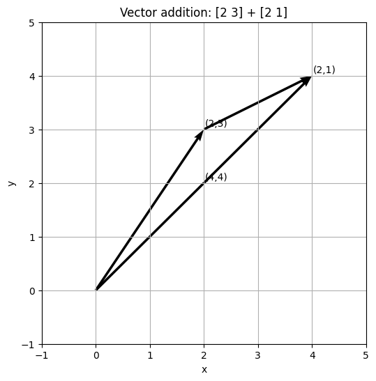 ## Subtracting Vectors Mathematically, subtracting vectors is just negative addition. But, geometrically, the procedure is different. In vector addition, the added vector starts at the head of the base vector. The answer is the line between the first tail and last head. In vector subtraction, the subtracted, or 'negative' vector, starts at the tail of the other vector. The resultant is the vector from the head of the subtracted, or negative, or subtrahend, vector to the head of the minuend vector. Vector subtraction: [2 3] - [2 1] ```python # Define the vector 'a' a = np.array([2, 3]) b = np.array([2, 1]) # Create a plot of the vector 'a' plt.close() plt.figure(figsize=(6, 6)) plt.quiver(0, 0, a[0], a[1], angles='xy', scale_units='xy', scale=1) plt.quiver(0, 0, b[0], b[1], angles='xy', scale_units='xy', scale=1) plt.quiver(b[0], b[1], a[0]-b[0], a[1]-b[1], angles='xy', scale_units='xy', scale=1) # Annotate the vector plt.annotate(f"a = ({a[0]}, {a[1]})", xy=(a[0], a[1]), xytext=(5, 5), textcoords="offset points", ha="center") plt.annotate(f"b = ({b[0]}, {b[1]})", xy=(b[0]+.5, b[1]+.1), ha="center") plt.annotate("a-b=(0, 2)", xy=(2.5,2), ha="center") plt.xlabel("X-axis") plt.ylabel("Y-axis") plt.title("Vector subtraction: [2 3] - [2 1]") plt.xlim(-1, max(abs(a))+1) plt.ylim(-1, max(abs(a))+1) plt.grid() plt.show() ``` 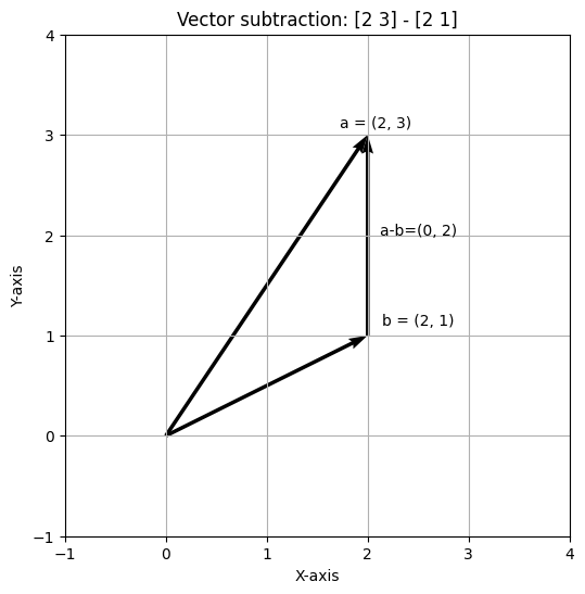 ## Averaging Vectors Averaging is sum then divide by N. Averaging vectors is to add them, then scalar multiply by 1/N vectors. ```python print("(", a, "+", b, ") * 1/N vectors") (a+b)*(1/2) ``` ``` ( [2 3] + [2 1] ) * 1/N vectors array([2., 2.]) ``` ## By hand: averaging [https://aibyhand.substack.com/p/w6-batch](https://aibyhand.substack.com/p/w6-batch) ```python (2+2+2+6)/4 ``` ``` 3.0 ``` ```python (1+1+1+1+1+1+1)/10 ``` ``` 0.7 ``` ```python np.mean([1,1,0,1,1,1,1,1,0,1]) ``` ``` 0.8 ``` ## Multiplying Vectors ```python print(a, "*", b) a*b ``` ``` [2 3] * [2 1] array([4, 3]) ``` ## Vector Transposition Matrices have **(row,column)** indices. Transposition swaps those indices. $\mathbf{m}^T_{i,j}=\mathbf{m}_{j,i}$ ## By hand: row and column @ alan yeh. ai by hand [https://aibyhand.substack.com/](https://aibyhand.substack.com/) ```python def m(*x): return np.array([[*x]]) def M(*x): return np.array([*x]) m(5,2).T!=m(5,2) ``` ``` array([[False, True], [ True, False]]) ``` ## Vector Dimensionality Vectors have either one row, or one column, depending on orientation. So, a 6D row vector $\mathbf{v}$ has indices $i=1$, $j=6$, or $\mathbf{m}_{1,6}$. ## Vector Broadcasting add a row to column vector ``` [[4] [5] [6]] + [[1 2 3]] array([[5, 6, 7], [6, 7, 8], [7, 8, 9]]) ``` ## Vector Magnitude The geometric length (magnitude) of a vector. Denoted like $\lVert\mathbf{v}\rVert$ The magnitude is the distance from the tail to the head of a vector, computed using the standard Euclidean distance formula: the square root of the sum of squared vector elements: $$\displaystyle\lVert\mathbf{v}\rVert=\sqrt{\sum{^n_i}=1v^2_i}$$ or $$\lVert\mathbf{v}\rVert^2=\sum{^n_i}=1v^2_i$$ or $$\lVert\mathbf{v}\rVert=\sqrt{\mathbf{v}^\top\mathbf{v}}$$ math.sqrt(np.dot(x.T, x)) ``` Dimensions: 6 Magnitude: 9.539392014169456 Magnitude: 9.539392014169456 ``` Euclidean distance is the straight-line distance between two points. In the plane, from $(x_1,y_1)$ to $(x_2,y_2)$, $$d=\sqrt{(x_2-x_1)^2+(y_2-y_1)^2}$$ That expression is the Pythagorean theorem. A right triangle has one square corner. The hypotenuse is the side across from that corner. If the other two sides, the legs, have lengths $a$ and $b$, then $$c^2=a^2+b^2$$ so the hypotenuse is $$c=\sqrt{a^2+b^2}$$ Each squared term in the distance is one leg: the horizontal step and the vertical step. The square root of their sum is the straight line. The magnitude of a vector is that same distance measured from the origin, the point $(0,0)$, where the tail sits. In $n$ dimensions the same idea stacks one squared step per axis: $$\lVert\mathbf{v}\rVert=\sqrt{v_1^2+v_2^2+\cdots+v_n^2}$$ A worked 3-4-5 triangle is under [The Dot Product and Vector Magnitude](#the-dot-product-and-vector-magnitude). ## Unit Vectors $$\lVert\mathbf{v}\rVert=1$$ Creating a unit vector: $$\mathbf{\widehat{v}}=\frac{1}{\lVert\mathbf{v}\rVert}\mathbf{v}$$ The set of infinite unit vectors is smaller than the set of infinite non-unit vectors. Here's why: Generate a small number of random points for each set Print the sets: a random non-unit vector ``` np.float64(5.322962650718925) ``` a random unit vector ``` np.float64(0.9999999999999999) ``` All unit vectors norm to 1, meaning they have a magnitude of 1. The set is bounded and closed. All non-unit vectors can have any magnitude. The set is unbounded and open. ## Crafting a unit vector from a nonunit vector $$\widehat{\mathbf{v}}=\frac{1}{\lVert\mathbf{v}\rVert}\mathbf{v}$$ Simply scalar multiply by the reciprocal of the vector norm. ```python a_unit_vector = 1/(np.linalg.norm(a))*a print(a) print(np.linalg.norm(a_unit_vector)) ``` ``` [[1 2 3]] 1.0 ``` ## Vector Dot Product Notations: $\mathbf{a}^\top\mathbf{b}$, $\mathbf{a \cdot b}$, $\langle \mathbf{a, b} \rangle$ $\mathbf{a}$ and $\mathbf{b}$ are vectors, and $a_i$ indicates the *i*th element of $\mathbf{a}$. The equation: $$\delta=\sum^n_{i=1}a_i b_i$$ So: $$\begin{bmatrix} 1 2 3 4\end{bmatrix}\cdot\begin{bmatrix}5 6 7 8\end{bmatrix}$$ $$=1\times5+2\times6+3\times7+4\times8$$ $$=5+12+21+32$$ $$=70$$ ### The Dot Product and Vector Magnitude Note, the Pythagorean theorem is a special case of the dot product. It's also related to vector magnitude and the cosine of the angle between two vectors. $c^2=a^2+b^2$ gives the length of the hypotenuse of a right triangle with sides of length $a$ and $b$. For a triangle with sides of length $3$ and $4$, and a hypotenuse of length $c$, the Pythagorean theorem is: $$c^2=3^2+4^2$$ $$c^2=9+16$$ $$\sqrt{c^2}=\sqrt{25}$$ $$c=5$$ Given a vector $\mathbf{x} = \begin{bmatrix}3\\4\end{bmatrix}$, the magnitude of the vector is: $$\lVert\mathbf{x}\rVert=\sqrt{3^2+4^2}$$ $$\lVert\mathbf{x}\rVert=\sqrt{9+16}$$ $$\lVert\mathbf{x}\rVert=\sqrt{25}$$ $$\lVert\mathbf{x}\rVert=5$$ So the magnitude of a vector is the hypotenuse of a right triangle with sides of length $a$ and $b$. And given the vector $\mathbf{x} = \begin{bmatrix}3\\4\end{bmatrix}$, squaring $a$ and $b$ is the same as applying the dot product to the vector with itself. $$\mathbf{x}^\top\mathbf{x}=\begin{bmatrix}3 & 4\end{bmatrix}\begin{bmatrix}3\\4\end{bmatrix}$$ $$\mathbf{x}^\top\mathbf{x}=3^2+4^2$$ $$\mathbf{x}^\top\mathbf{x}=9+16$$ $$\mathbf{x}^\top\mathbf{x}=25$$ $$\mathbf{x}^\top\mathbf{x}=\sqrt{25}$$ $$\mathbf{x}^\top\mathbf{x}=5$$ So generally we have $$\sqrt{\mathbf{x}^\top\mathbf{x}}=\lVert\mathbf{x}\rVert$$ So the dot product of a vector with itself is the square of the magnitude of the vector. And the magnitude of a vector is the square root of the dot product of the vector with itself. $$\lVert\mathbf{x}\rVert=\sqrt{\mathbf{x}^\top\mathbf{x}}$$ ### The Dot Product and the Angle Between Two Vectors The angle $\theta$ between two vectors is related to the dot product by the formula: $$\mathbf{x}^\top\mathbf{y}=\lVert\mathbf{x}\rVert\lVert\mathbf{y}\rVert\cos(\theta)$$ We solve the equation to get the cosine of the angle between two vectors: $$\cos(\theta)=\frac{\mathbf{x}^\top\mathbf{y}}{\lVert\mathbf{x}\rVert\lVert\mathbf{y}\rVert}$$ Given $\mathbf{x}=\begin{bmatrix}2\\-3\end{bmatrix}$ and $\mathbf{y}=\begin{bmatrix}3\\2\end{bmatrix}$: $$= \frac{\begin{bmatrix}2 & -3\end{bmatrix}\begin{bmatrix}3\\2\end{bmatrix}}{\sqrt{2^2+(-3)^2}\sqrt{3^2+2^2}}\\ = \frac{0}{13}\\ = 0 $$ Dot products are 0 when the vectors are perpendicular. Note $\theta=cos^{-1}(0)=90^\circ$. $$\mathbf{x}\perp\mathbf{y} \iff \mathbf{x}^\top\mathbf{y}=0$$ Generalizing the dot product to an arbitary number of dimensions is called the inner product: $$\mathbf{a}^\top\mathbf{b}=\sum^n_{i=1}a_i b_i$$ ```python a = np.array([1,2,3,4]) b = np.array([5,6,7,8]) print(np.dot(a,b)) print(a@b) # the same thing ``` ``` 70 70 ``` You can scalar multiply one vector, which scales the dot product by the same amount. ```python scalar1 = 10 print(a*scalar1@b) # can be applied to one vector print((a@b)*scalar1) # or the dot product itself scalar1 = -10 # a negative scalar preserves the magnitude but switches the sign print(a*scalar1@b) print((a@b)*scalar1) ``` ``` 700 700 -700 -700 ``` ## The Dot Product is Distributive $$\mathbf{a}^\top(\mathbf{b}+\mathbf{c})=\mathbf{a}^\top\mathbf{b}+\mathbf{a}^\top\mathbf{c}$$ ```python a = np.array([0,1,2]) b = np.array([3,4,5]) c = np.array([6,7,8]) print(np.dot(a, b+c)) print(np.dot(a,b) + np.dot(a,c)) ``` ``` 37 37 ``` ## Geometric Definition of the Vector Dot Product $$\alpha = \cos(\theta_{\mathbf{v},\mathbf{w}}) \lVert\mathbf{v}\rVert\,\lVert\mathbf{w}\rVert$$ or $$\cos(\theta_v,_w)=\frac{\mathbf{v}^\top\mathbf{w}}{\lVert\mathbf{v}\rVert\,\lVert\mathbf{w}\rVert}$$ The product of the magnitude of the two vectors, scaled by the cosine of the angle between them. Cosine similarity is that cosine, the fraction already written above: $$\frac{\mathbf{x}^\top\mathbf{y}}{\lVert\mathbf{x}\rVert\,\lVert\mathbf{y}\rVert}$$ Cosine distance is one minus that fraction: $$1-\frac{\mathbf{x}^\top\mathbf{y}}{\lVert\mathbf{x}\rVert\,\lVert\mathbf{y}\rVert}$$ The pairs of numbers below are those two quantities for each pair of vectors. the spatial cosine similarity the spatial cosine distance ``` [0 1 2] [3 4 5] Cosine similarity 0.8854377448471461 Cosine distance 0.11456225515285379 ``` the spatial cosine similarity the spatial cosine distance ``` [0 1 2] [6 7 8] Cosine similarity 0.8426548012644084 Cosine distance 0.1573451987355916 ``` angle theta between two vectors ``` Cosine angle 0.5686015478708155 Cosine angle 32.58° Cosine angle 32.58° ``` scalar projection from the angle theta the length of the projection of vector a onto vector b The scalar projection is that length as a single number. If $\theta$ is the angle between $\mathbf{a}$ and $\mathbf{b}$, the length of the shadow of $\mathbf{a}$ cast onto $\mathbf{b}$ is $$\lVert\mathbf{a}\rVert\cos\theta=\frac{\mathbf{a}^\top\mathbf{b}}{\lVert\mathbf{b}\rVert}$$ The orthogonal projection section below solves for the scalar $\beta$ that places the shadow of $\mathbf{b}$ onto $\mathbf{a}$. That shadow vector is $\beta$ times $\mathbf{a}$, and $\beta$ times the length of $\mathbf{a}$ is this same kind of length. ``` Scalar projection a -> b: 1.884233417193793 ``` ## Orthogonal Vectors Have a Zero Dot Product *two vectors are orthogonal if:* - two vectors have a dot product of zero - two vectors meet at 90 degree angles Perpendicular vectors ```python # TODO: move to 'Orthogonal Vectors Have a Zero Dot Product' # if the dot product is 0 # the vectors are perpendicular pvec2([4,2],[-1,2],title='Perpendicular vectors') np.dot([4,2],[-1,2]) ``` 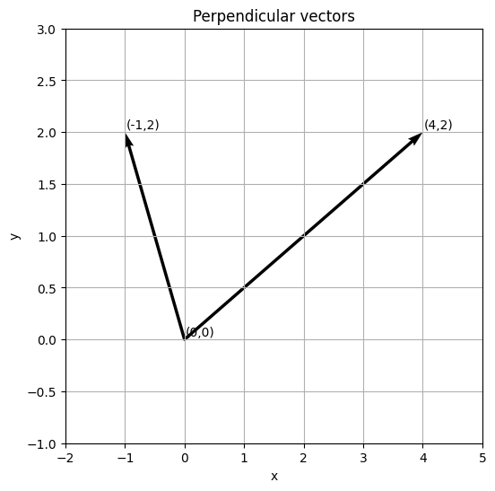 Not perpendicular ```python # TODO: move to 'Orthogonal Vectors Have a Zero Dot Product' pvec2([1,2],[3,1], title='Not perpendicular') np.dot([1,2],[3,1]) ``` 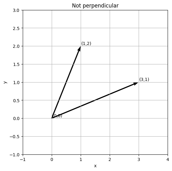 ## Hadamard Multiplication Element-wise mutliplication $$\begin{bmatrix} 5\\ 4\\ 8\\ 2\end{bmatrix} \odot \begin{bmatrix} 1\\ 0\\ .5\\ -1\end{bmatrix} = \begin{bmatrix} 5\\ 0\\ 4\\ -2\end{bmatrix}$$ ```python a = np.array([5,4,8,2]) b = np.array([1,0,0.5, -1]) a*b ``` ``` array([ 5., 0., 4., -2.]) ``` ## Outer Product $$\begin{bmatrix} a\\ b\\ c\end{bmatrix} \begin{bmatrix}d\, e\end{bmatrix}=\begin{bmatrix}ad\, ae\\ bd\, be\\cd\, ce\end{bmatrix}$$ Denoted $\mathbf{v}\mathbf{w}^\top$ because we assume all vectors are columnar until indicated, so the outer product is column vector $\mathbf{v}$ times the row vector $\mathbf{w}$. ```python a = np.array([1,2,3]) b = np.array([4,5]) print(np.outer(a,b)) ``` ``` [[ 4 5] [ 8 10] [12 15]] ``` ```python for _a in a: for _b in b: print(_a * _b) ``` ``` 4 5 8 10 12 15 ``` ## Orthogonal Vector Projection We want to project a point at the head of vector $\mathbf b$ onto vector $\mathbf a$ with minimum distance. This will result in a vector that intersects vector $\mathbf a$ at a right angle. The point at which the projection intersects $\mathbf{a}$ will be called $\beta$. And the vector from the head of $\mathbf{b}$ to $\beta$ will be called $\mathbf{b}-\beta\mathbf{a}$. Vector ```python # Define the vector 'a' a = np.array([2, 3]) b = np.array([2, 1]) beta = np.dot(a,b)/np.dot(a,a) # the orthogonal projection from the head of b, to a projected_beta = a*beta # Create a plot of the vector 'a' plt.close() plt.figure(figsize=(6, 6)) plt.quiver(0, 0, a[0], a[1], angles='xy', scale_units='xy', scale=1) plt.quiver(0, 0, b[0], b[1], angles='xy', scale_units='xy', scale=1) plt.quiver(b[0], b[1], projected_beta[0]-b[0], projected_beta[1]-b[1], angles='xy', scale_units='xy', scale=1) # Annotate the vector plt.annotate(f"a = ({a[0]}, {a[1]})", xy=(a[0], a[1]), xytext=(5, 5), textcoords="offset points", ha="center") plt.annotate(f"b = ({b[0]}, {b[1]})", xy=(b[0]+.25, b[1]), xytext=(5, 5), textcoords="offset points", ha="center") plt.xlabel("X-axis") plt.ylabel("Y-axis") plt.title("Vector 'a', 'b', and the orthogonal projection vector") plt.xlim(-1, max(abs(a))+1) plt.ylim(-1, max(abs(a))+1) plt.grid() plt.show() ```  The dot product between orthogonal vectors is 0. And we know the projection from the head of $\mathbf b$ will create an orthogonal vector. So, the projection vector is orthogonal to $\beta$ on vector $\mathbf{a}$, and the dot product is zero. Thus, $$\mathbf{a}^\top(\mathbf{b}-\beta\mathbf{a})=0$$ We use the distributive property of dot products and apply algebra to solve for zero. $$\mathbf{a}^\top\mathbf{b}-\beta\mathbf{a}^\top\mathbf{a}=0$$ $$\beta\mathbf{a}^\top\mathbf{a}=\mathbf{a}^\top\mathbf{b}$$ $$\beta=\frac{\mathbf{a}^\top\mathbf{b}}{\mathbf{a}^\top\mathbf{a}}$$ Which is to say, $\beta$ is the quotient of the dot product of column vector $\mathbf{a}$ and row vector $\mathbf{b}$ over the dot product of column vector $\mathbf{a}$ and row vector $\mathbf{a}$. It scales vector $\mathbf{a}$. ```python print(a) print(b) print(np.dot(a,b)/np.dot(a,a)) print(a*beta) # the resulting vector is colinear with vector a, and the head is at the point which is closest to the head of vector b. ``` ``` [2 3] [2 1] 0.5384615384615384 [1.07692308 1.61538462] ``` ## Orthogonal Vector Decomposition Given a vector $\mathbf{t}$, we want to decompose it into the sum of two vectors that are orthogonal and parallel to a reference vector $\mathbf{r}$. This will produce two vectors: a parallel vector $\mathbf{t\parallel r}$, and a perpendicular vector $\mathbf{t\bot r}$. So we must find a vector that is parellel to $\mathbf{r}$. Any scaled version of $\mathbf{r}$ is parallel, so we find $\mathbf{t\parallel r}$ by applying orthogonal projection. $$\mathbf{t\parallel r} = \mathbf{r}\frac{\mathbf{t}^\top\mathbf{r}}{\mathbf{r}^\top\mathbf{r}}$$ Because vector $\mathbf{t\parallel r}$ is a scaled version of $\mathbf{r}$, it could be thought of as $\beta\mathbf{r}$. Rather than compute just the scalar, like in projection, we compute the scaled vector. The perpendicular and parallel vectors $\mathbf{t\parallel r}$ and $\mathbf{t\bot r}$ will sum to the target vector $\mathbf{t}$, so using algebra: $$\mathbf{t}=\mathbf{t\bot r}+\mathbf{t\parallel r}$$ $$\mathbf{t\bot r}=\mathbf{t-t\parallel r}$$ Vector Decomposition ```python t = np.array([2.58,1.44]) r = np.array([2.41,2.22]) parallel_r = r*(np.dot(t.T, r))/(np.dot(r.T,r)) perpendicular_r = t-parallel_r plt.close() plt.figure(figsize=(6, 6)) plt.quiver(0, 0, t[0], t[1], angles='xy', scale_units='xy', scale=1) plt.quiver(0, 0, r[0], r[1], angles='xy', scale_units='xy', scale=1) plt.quiver(0, 0, parallel_r[0], parallel_r[1], angles='xy', scale_units='xy', scale=1) plt.quiver(0, 0, perpendicular_r[0], perpendicular_r[1], angles='xy', scale_units='xy', scale=1) plt.annotate(f"t = ({round(t[0],2)}, {round(t[1],2)})", xy=(t[0], t[1]), xytext=(5, 5), textcoords="offset points", ha="center") plt.annotate(f"r = ({round(r[0],2)}, {round(r[1],2)})", xy=(r[0], r[1]), xytext=(5, 5), textcoords="offset points", ha="center") plt.xlabel("X-axis") plt.ylabel("Y-axis") plt.title("Vector Decomposition") plt.xlim(-1.5, 3.5) plt.ylim(-1.5, 3.5) plt.tight_layout() plt.grid() plt.show() ```  ## Vector Sets Denoted like $V = \{\mathbf{v_1,...,v_n}\}$ ## Linear Weighted Combination Scalar-vector multiplication and addition: take a set of vectors, multiply each vector by a scalar, then add them to product a single vector. $\mathbf{w}=\lambda_1\mathbf{v}_1+\lambda_2\mathbf{v}_2+...+\lambda_n\mathbf{v}_n$ All the vectors have to have the same dimensionality. $$\lambda_1=1,\,\,\lambda_2=2,\,\,\lambda_3=-3\qquad \mathbf{v}_1=\begin{bmatrix}4\\ 5\\ 1\end{bmatrix}, \mathbf{v}_2=\begin{bmatrix}-4\\ 0\\ -4\end{bmatrix}, \mathbf{v}_3=\begin{bmatrix}1\\ 3\\ 2\end{bmatrix}$$ $$\mathbf{w}=\lambda_1\mathbf{v}_1+\lambda_2\mathbf{v}_2+\lambda_3\mathbf{v}_3=\begin{bmatrix}-7\\ -4\\ -13\end{bmatrix}$$ ```python l1 = 1 l2 = 2 l3 = -3 v1 = np.array([4,5,1]) v2 = np.array([-4,0,-4]) v3 = np.array([1,3,2]) l1*v1 + l2*v2 + l3*v3 ``` ``` array([ -7, -4, -13]) ``` the tinygrad way ``` array([ -7, -4, -13]) ``` ## Linear Independence A vector set is *linearly dependent* if at least one vector in the set can be expressed as a linear weighted combination of other vectors in that set. If no vectors in the set can be expressed as a linear weighted combination, the set is *linearly independent*. $$V = \begin{Bmatrix}\begin{bmatrix}1\\ 3\end{bmatrix},\begin{bmatrix}2\\ 7\end{bmatrix}\end{Bmatrix}\qquad S = \begin{Bmatrix}\begin{bmatrix}1\\ 3\end{bmatrix},\begin{bmatrix}2\\ 6\end{bmatrix}\end{Bmatrix}$$ Vector set $V$ is *linearly independent* because neither vector can be expressed as the linear weighted combination of the other. Vector set $S$ is *linearly dependent* because one vector **can** be expressed as the linear weighted combination of the other. There is an infinite number of potential linear combinations for set $S$, two of which are $\mathbf{s}_1=0.5s_2$ and $\mathbf{s}_2=2s_1$. ```python print(np.array([2,6])*0.5) print(np.array([1,3])*2) ``` ``` [1. 3.] [2 6] ``` So linear dependence can be expressed as $\mathbf{0}=\lambda_1\mathbf{v}_1+\lambda_2\mathbf{v}_2+...+\lambda_n\mathbf{v}_n,\quad\lambda\in\mathbb{R}$. If you can find some $\lambda$s that make the equation true, the set is linearly dependent. But, usually the equation is constrained to non-trivial solutions. That is, at least one $\lambda\ne0$. This constraint can be incorporated into the equation: $$\mathbf{0}=\mathbf{v}_1+...+\frac{\lambda_n}{\lambda_1}\mathbf{v}_n,\quad\lambda\in\mathbb{R},\,\lambda_1\ne0$$ Linear independence means the vectors contain information. ## Subspace and Span For any finite set of vectors, there are an infinite number of ways to linearly combine them using different weights, creating a *vector subspace*. The mechanism for combining all possible linear weighted combinations is the *span* of the vector set. Take, for instance: $$V = \begin{Bmatrix}\begin{bmatrix}1\\ 3\end{bmatrix}\end{Bmatrix}$$ A Vector (black) and the subspace it spans (gray) ```python a = np.array([1,3]) scaled_a = a*5 negative_scaled_a = scaled_a * -1 plt.close() plt.figure(figsize=(6, 6)) plt.quiver(0, 0, a[0], a[1], angles='xy', scale_units='xy', scale=1) plt.quiver(0, 0, scaled_a[0], scaled_a[1], angles='xy', scale_units='xy', scale=1, color="grey", alpha=0.5) plt.quiver(0, 0, negative_scaled_a[0], negative_scaled_a[1], angles='xy', scale_units='xy', scale=1, color="grey", alpha=0.5) plt.annotate(f"a = ({round(a[0],2)}, {round(a[1],2)})", xy=a, xytext=(3, 3), textcoords="offset points", ha="center") plt.xlabel("X-axis") plt.ylabel("Y-axis") plt.title("A Vector (black) and the subspace it spans (gray)") plt.xlim(-1, 2) plt.ylim(-2, 5) plt.tight_layout() plt.grid() plt.show() ```  Now, a set of two vectors in $\mathbb{R}^3:$ $$V = \begin{Bmatrix}\begin{bmatrix}1\\0\\2\end{bmatrix},\begin{bmatrix}-1\\1\\2\end{bmatrix}\end{Bmatrix}$$ (FIX) Vectors in R^3 and the subspace they span ```python # TODO: fix the graph the subspace plane a = np.array([1,0,2]) b = np.array([-1,1,2]) # no idea how to graph the 3d subspace, and this isn't correct X = np.linspace(a[0], b[0], 10) Y = np.linspace(a[1], b[1], 10) X,Y = np.meshgrid(X,Y) Z = X * a[0] + Y * a[1] + (a[2] - a[0]*b[0] - a[1]*b[1]) / b[2] plt.close() ax = plt.figure(figsize=(6, 6)).add_subplot(projection='3d') ax.quiver(0,0,0,a[0],a[1],a[2]) ax.quiver(0,0,0,b[0],b[1],b[2]) ax.plot_surface(X, Y, Z) plt.title("(FIX) Vectors in R^3 and the subspace they span") ax.set_xlim(-2,2) ax.set_ylim(-2,2) ax.set_zlim(-2,2) plt.tight_layout() plt.grid() plt.show() ```  Points along a random 2D vector subspace ```python # randomized points along a 2D vector subspace # these points lie along a half-open interval [-4,4) of the vector subspace, based on the vector = [1 3] # there are an infinite number of potential points vector_set = np.array([1,3]) random_scalars = np.random.uniform(-4,4,100) subspace_points_x = [scalar*vector_set[0] for scalar in random_scalars] subspace_points_y = [scalar*vector_set[1] for scalar in random_scalars] plt.close() plt.figure(figsize=[6,6]) plt.scatter(subspace_points_x, subspace_points_y) plt.title('Points along a random 2D vector subspace') plt.xlim(-4,4) plt.ylim(-4,4) plt.grid() ``` 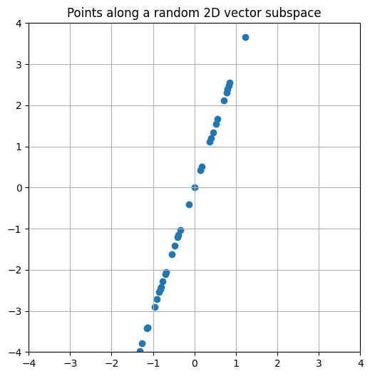 Points along a random 3D vector subspace ```python # randomized points along a 3D vector subspace # all the points lie along the same 3D plane when graphed # TODO: graph the plane vector_set_v1 = np.array([3,5,1]) vector_set_v2 = np.array([0,2,2]) random_scalars_1 = np.random.uniform(-4,4,100) random_scalars_2 = np.random.uniform(-4,4,100) plt.close() p1x, p1y, p1z = [],[],[] for scalar in random_scalars_1: p1x.append(scalar*vector_set_v1[0]) p1y.append(scalar*vector_set_v1[1]) p1z.append(scalar*vector_set_v1[2]) p2x, p2y, p2z = [],[],[] for scalar in random_scalars_2: p1x.append(scalar*vector_set_v2[0]) p1y.append(scalar*vector_set_v2[1]) p1z.append(scalar*vector_set_v2[2]) ax = plt.figure(figsize=(6, 6)).add_subplot(projection='3d') ax.scatter(p1x, p1y, p1z) ax.scatter(p2x, p2y, p2z) plt.title('Points along a random 3D vector subspace') plt.xlim(-4,4) plt.ylim(-4,4) ax.view_init(-20) plt.grid() ``` 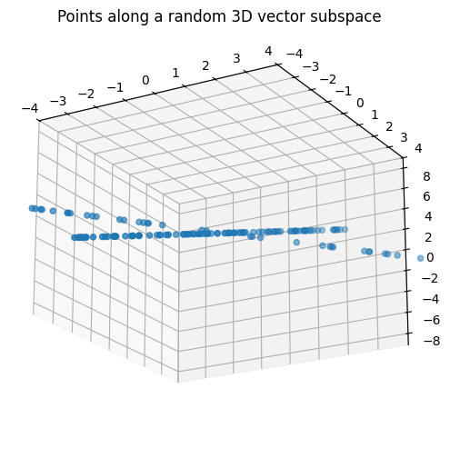 3 vectors that lie on a plane ```python # TODO: Create pvec function for R^3 space # compute u+v+w and 2u+2v+w. # How do you know u,v,w lie in a plane? u = np.array([1,2,3]) v = np.array([-3,1,-2]) w = np.array([2,-3,-1]) pvec3(u,v,w, title='3 vectors that lie on a plane') ``` 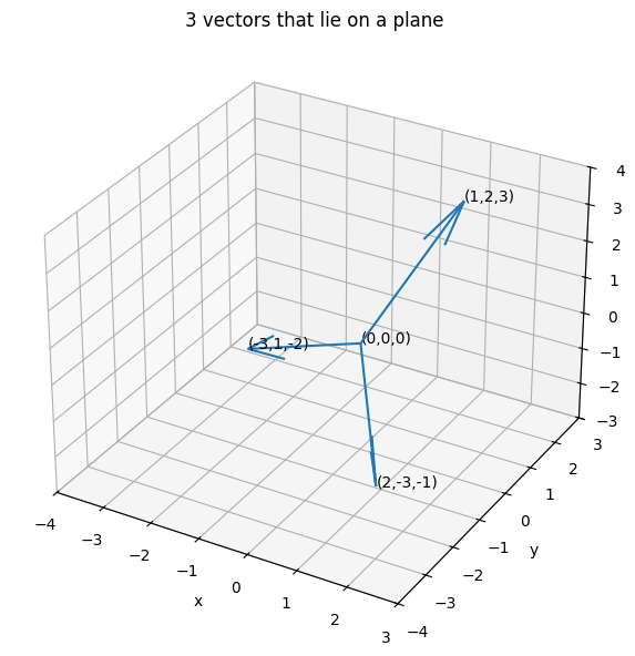 2 vectors that lie on a plane in R^3 ```python u = np.array([3,5,1]) v = np.array([0,2,2]) pvec3(u,v, title='2 vectors that lie on a plane in R^3') ``` 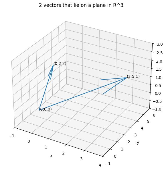 ## Basis A *basis* is a set of rulers used to describe the information in a matrix. A familiar basis set is the Cartesian axis: the standard XY (2D) or XYZ (3D) plane commonly used in graphing. The basis for 2D and 3D Cartesian graphs are: $$S_2=\begin{Bmatrix}\begin{bmatrix}1\\0\end{bmatrix},\begin{bmatrix}0\\1\end{bmatrix}\end{Bmatrix}\qquad S_3=\begin{Bmatrix}\begin{bmatrix}1\\0\\0\end{bmatrix},\begin{bmatrix}0\\1\\0\end{bmatrix},\begin{bmatrix}0\\0\\1\end{bmatrix}\end{Bmatrix}$$ Cartesian basis sets comprise vectors that are mutually orthogonal and unit length. It's often called the *standard basis set*. Here, we define a different basis set for illustration. $$T=\begin{Bmatrix}\begin{bmatrix}3\\1\end{bmatrix},\begin{bmatrix}-3\\1\end{bmatrix}\end{Bmatrix}$$ Now consider the following graph: The difference between basis sets ```python basis = np.array([[3,1],[-3,1]]) plt.close() plt.figure(figsize=(6, 6)) plt.plot(-6, 2, marker='s', markersize=10) plt.plot(3, 1, marker='o', markersize=10) plt.plot([0,1],[0,0], linewidth=4, color='black') plt.plot([0,0],[1,0], linewidth=4, color='black') plt.plot([0,3],[0,1], linewidth=4, color='red', linestyle='dotted') plt.plot([0,-3],[0,1], linewidth=4, color='red', linestyle='dotted') # plt.annotate(f"a = ({round(a[0],2)}, {round(a[1],2)})", xy=a, xytext=(3, 3), textcoords="offset points"\ plt.xlabel("X-axis") plt.ylabel("Y-axis") plt.title("The difference between basis sets") plt.xlim(-7,7) plt.ylim(-7,7) plt.tight_layout() plt.grid() plt.show() ``` 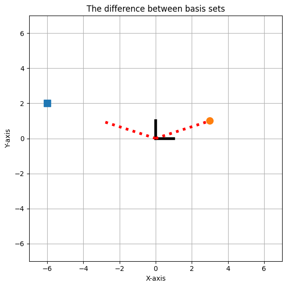 In the basis set $S_2$, the points above are $p=(3,1),\,q=(-6,2)$. We can express these points as the linear combination of the basis vector $S$: $$S=\begin{Bmatrix}\begin{bmatrix}1\\0\end{bmatrix},\begin{bmatrix}0\\1\end{bmatrix}\end{Bmatrix} \in\mathbb{R}^2$$ $$p=3\mathbf{s}_1+1\mathbf{s}_2,\,q=-6\mathbf{s}_1+2\mathbf{s}_2$$ If the basis set were: $$T=\begin{Bmatrix}\begin{bmatrix}3\\1\end{bmatrix},\begin{bmatrix}-3\\1\end{bmatrix}\end{Bmatrix}$$ the same points above could be expressed as: $$p=1\mathbf{t}_1+0\mathbf{t}_2,\,q=0\mathbf{t}_1+2\mathbf{t}_2$$ or $$p=\mathbf{t}_1,\,q=2\mathbf{t}_2$$ ## Pearson correlation coefficient Before the correlation coefficient can be calculated the data needs to be normalized to the expected range -1 to +1. First, *mean center each variable*. It means subtracting the average value from each data value. Then, *divide the dot product by the product of the vector norms*. Divisive normalization cancels the measurement units and scales the maximum possible correlation magnitude to $|1|$. The formula for Pearson correlation coefficient: $$\rho=\frac{\sum^n_{i=1} (x_i-\bar{x})(y_i-\bar{y})}{\sqrt{\sum^n_{i=1} (x_i-\bar{x})^2}\sqrt{\sum^n_{i=1} (y_i-\bar{y})^2}}$$ Once the variables are normalized, the equation can be rewritten as: $$\rho=\frac{\widetilde{\mathbf{x}}^\top\widetilde{\mathbf{y}}}{\lVert\mathbf{\widetilde{x}}\rVert\,\lVert\mathbf{\widetilde{y}}\rVert}$$ which is, to say, that the Pearson correlation coefficient is the dot product of two mean-centered variables, normalized by the magnitudes of the variables. ```python x = np.array([0,1,2,5]) y = np.array([100,101,102,103]) x = x-np.mean(x) y = y-np.mean(y) pcc = np.dot(x.T,y) / ((np.linalg.norm(x)) * np.linalg.norm(y)) print('Pearson correlation coefficient:', round(pcc,5)) ``` ``` Pearson correlation coefficient: 0.95618 ``` ```python scipy.stats.pearsonr(x,y) ``` ``` PearsonRResult(statistic=np.float64(0.956182887467515), pvalue=np.float64(0.04381711253248488)) ``` correlation between different vectors ```python # correlation between different vectors a = np.linspace(0,10,10) b = a c = a**2 d = 2**a a2 = np.linspace(0,11,11) e = [math.log(int(x)) for x in a2 if x > 0] f = [math.log(int(x))*x for x in a2 if x > 0] g = [math.factorial(int(x)) for x in a2 if x > 0] l = pd.Series([i for i in range(10)]) q = pd.Series([i**2 for i in range(10)]) e = pd.Series([2**i for i in range(10)]) logn = pd.Series([math.log(int(x)) for x in a2 if x > 0]) nlogn = pd.Series([math.log(int(x))*x for x in a2 if x > 0]) f = pd.Series([math.factorial(i) for i in range(10)]) df = pd.DataFrame([logn,l,nlogn,q,e,f], index=["logarithmic","linear","n log n","quadratic","exponential","factorial"]) corr_df = df.copy() df = df.style.set_caption("Vectors computed from functions f(x) where x = [0,10]") display(df) plt.close() plt.figure(figsize=[4,4]) plt.plot(a[:6],logn[:6],label="logarithmic") plt.plot(a[:6],b[:6],label="linear") plt.plot(a[:6],nlogn[:6],label="n log n") plt.plot(a[:6],c[:6],label="quadratic") plt.plot(a[:6],d[:6],label="exponential") plt.plot(a[:5],g[:5],label="factorial") plt.xlabel("input integer") plt.ylabel("output value") plt.grid() plt.legend(fontsize="x-small") plt.show() corr_df = corr_df.T.corr() corr_df = corr_df.style.set_caption("Correlation between vectors") display(corr_df) ``` 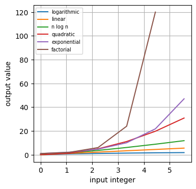 Mean-centering variables is a step in the correlation equation, illustrated below ```python # Mean-centering variables is a step in the # correlation equation, illustrated below x = np.random.rand(5,10) y = np.random.rand(5,10) # can also be done this way # fig, axs = plt.subplots(1,2) # axs[0].scatter(x,y) plt.close() fig, (ax1, ax2) = plt.subplots(1,2, figsize=[3,3]) fig.subplots_adjust(left=.0, right=2.5) ax1.scatter(x,y) ax1.set_xlim(-1,1) ax1.set_ylim(-1,1) ax1.set_title("random variables") ax1.grid() ax2.scatter(x-np.mean(x), y-np.mean(y)) ax2.set_xlim(-1,1) ax2.set_ylim(-1,1) ax2.set_title("mean-centered") ax2.grid() ``` 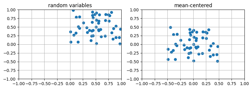 ## By hand: mean centering ```python def cen0(x): mean = np.mean(x) return x-mean ``` ```python mu = np.mean([-1,1,1,-1]) print([-1,1,1,-1]-mu) ``` ``` [-1. 1. 1. -1.] ``` ```python mu = np.mean([-2,0,-4,-2]) print([-2,0,-4,-2]-mu) ``` ``` [ 0. 2. -2. 0.] ``` ```python cen0([3,6,3,0]) ``` ``` array([ 0., 3., 0., -3.]) ``` ```python cen0([1,4,-1,0]) ``` ``` array([ 0., 3., -2., -1.]) ``` As the Big O complexity vectors above grow, their respective correlation coefficients describe how those vectors move apart, e.g. the correlation between the `log n` and `factorial` vectors is the smallest coefficient, as those vectors grow apart the fastest. ## Correlation vs. Cosine Similarity Both give measures of similarity, but start from different assumptions. In Pearson, [0,1,2,3] and [100,101,102,103] are perfectly correlated $(\rho=1)$. But the cosine similarity is .808, because the variables are a different numeric scale. Pearson correlation, written above, subtracts each variable's average before that same fraction. The average is the ordinary mean: add the entries and divide by how many there are. Cosine similarity uses the entries as they stand. Adding 100 to every entry of $[0,1,2,3]$ leaves the Pearson correlation at 1, and moves the cosine similarity to 0.808. The cosine distance between those two vectors is $1-0.808=0.192$. ## Cosine Distance ```python print("cosine distance from", a) df = pd.DataFrame([scipy.spatial.distance.cosine(a,func) for func in [logn,l,nlogn,q,e,f]], index=["logarithmic","linear","n log n","quadratic","exponential","factorial"]).T df.index = ["cosine distance"] df ``` ``` cosine distance from [ 0. 1.11111111 2.22222222 3.33333333 4.44444444 5.55555556 6.66666667 7.77777778 8.88888889 10. ] logarithmic linear n log n quadratic exponential \ cosine distance 0.018452 2.220446e-16 0.005042 0.031301 0.179017 factorial cosine distance 0.411332 ``` ## K-means Clustering 1. Initialize $k$ centroids. 2. Compute the Euclidean distance between each data observation (sample) and each centroid. 3. Assign each data observation to the group with the closest centroid. 4. Update each centroid as the average of all data observations assigned to that centroid. 5. Repeat steps 2-4 until a convergence criteria is satisfied, or for $N$ iterations. random data for k-means clustering ```python ## Create data nPerClust = 50 # blur around centroid (std units) blur = 1 # XY centroid locations A = [ 1, 1 ] B = [ -3, 1 ] C = [ 3, 3 ] # generate data a = [ A[0]+np.random.randn(nPerClust)*blur , A[1]+np.random.randn(nPerClust)*blur ] b = [ B[0]+np.random.randn(nPerClust)*blur , B[1]+np.random.randn(nPerClust)*blur ] c = [ C[0]+np.random.randn(nPerClust)*blur , C[1]+np.random.randn(nPerClust)*blur ] # concatenate into a matrix data = np.transpose(np.concatenate((a,b,c),axis=1)) plt.close() plt.figure(figsize=(3, 3)) plt.scatter(data[:,0], data[:,1]) # array[row_start:row_stop:row_step, col_start:col_stop:col_step] plt.title("random data for k-means clustering") plt.grid() plt.show() ``` 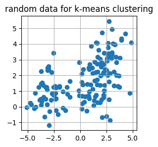 STEP 1 use a random choice of 3 indices to select 3 random centroids ``` [[-3.02773309 2.57701021] [ 3.9243609 4.33671332] [ 3.46027411 2.00236922]] ``` The Euclidean distance formula for one data observation and centroid can be computed as: $$\delta_{i,j}=\sqrt{(d^x_i-c^x_j)^2+(d^y_i-c^y_j)^2}$$ where $\delta_{i,j}$ is the distance from data observation $i$ ot centroid $j$, $d^x_i$ is feature $x$ of the $i$th data observation, and $c^x_j$ is the $x$-axis coordinate of centroid $j$. Each subtracted pair is one leg of a right triangle: the horizontal gap between the point and the centroid, and the vertical gap. The square root of the sum of those squares is the hypotenuse, the straight-line distance. A larger distance has a larger square, so the centroid with the smallest squared distance is the same centroid the square root would have picked. STEP 2 compute the distances from data observations to centroids Data is size 150 x 2 (observations by features) and centroids[ci, :] is 1 x 2 (cluster ci by features). Python broadcasts the cluster centroids 150 times, subtracting the centroid from each data observation. Then the exponent operation **2 is applied element-wise, and the axis=1 tells Python to sum across the columns, separately per row. So the output of np.sum() is a 150 x 1 array that encodes the Euclidean distance from each point to centroid ci. The square root of the original Euclidean distance formula isn't used because distance and squared distance are monotonic, so the square root is skipped to save on computation. STEP 3 assign to groups (classify) based on minimum distances recompute and migrate centroids Here we loop over $k$ clusters, and use indexing to find al the data points assigned to each cluster. ```python # run the procedure, starting with computing the distances from data to centroids # until some convergence criteria plt.close() plt.figure(figsize=[6,6]) plt.scatter(data[:,0], data[:,1]) plt.scatter(centroids[:,0], centroids[:,1]) plt.title('k-means clustering') plt.grid() plt.show() ``` 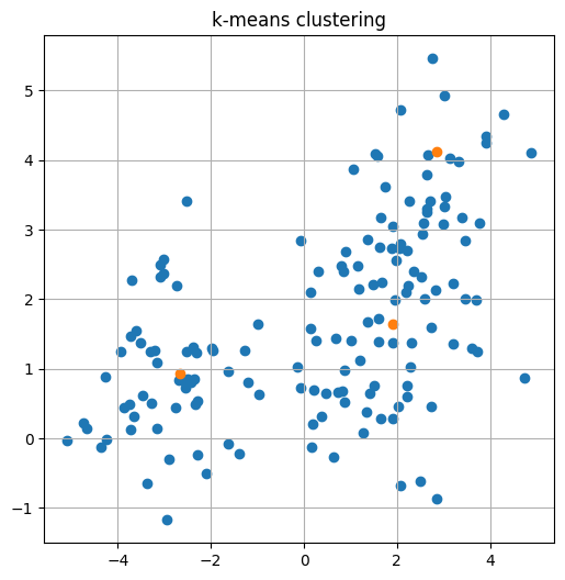 ## Filtering and Feature Detection with a kernel and the dot product A kernel here is a short fixed vector, a small pattern. At each position along the signal, the dot product of the kernel with the stretch of signal under it is large when that stretch points the same way as the pattern. The kernel $[-1,1]$ is large where the signal steps up, and large with the opposite sign where the signal steps down. a random signal with plateau function use the dot product to detect changes in the signal ```python # a random signal with plateau function signal = np.zeros(100) modulation = np.random.choice(range(89)) signal[modulation:modulation+10] = 1 # use the dot product to detect changes in the signal kernel = np.array([-1,1]) detected_features = np.zeros(len(signal)) for step in range(len(signal)-1): _ = np.array([signal[step], signal[step+1]]) detected_features[step+1] = np.dot(kernel, _) plt.close() fig, (ax1, ax2) = plt.subplots(1,2, figsize=[10,3]) ax1.plot(signal) ax2.plot(detected_features) ax1.set_ylim(-10,10) ax2.set_ylim(-10,10) ax1.set_title('signal') ax2.set_title('edge detection') ax1.grid(); ax2.grid() ``` 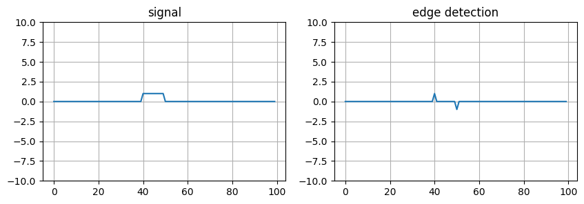 ## Signal smoothing with a kernel and dot product The same dot product, with a kernel shaped like a low hill. Each output sample is a weighted blend of the samples around it, so a spike is pulled toward its neighbors. a random signal with plateau function creates an obvious magnitude spike for illustration ```python # a random signal with plateau function signal = np.random.randn(100) # creates an obvious magnitude spike for illustration signal[50:60] = signal[50:60]+2 # use the dot product to detect changes in the signal kernel = np.array([0, 0.1, 0.3, 0.8, 1, 0.8, 0.3, 0.1, 0]) klen = len(kernel) half_klen = klen // 2 smoothed_signal = signal.copy() for t in range(half_klen+1,len(signal)-half_klen): smoothed_signal[t] = np.dot(kernel,signal[t-half_klen-1:t+half_klen]) plt.close() fig, (ax1, ax2, ax3) = plt.subplots(1, 3, figsize=[10,3]) ax1.plot(kernel) ax2.plot(signal) ax3.plot(smoothed_signal) ax1.set_ylim(-10,10) ax2.set_ylim(-10,10) ax3.set_ylim(-10,10) ax1.set_title('kernel') ax2.set_title('signal') ax3.set_title('smoothed signal') ax1.grid(); ax2.grid(); ax3.grid() ``` 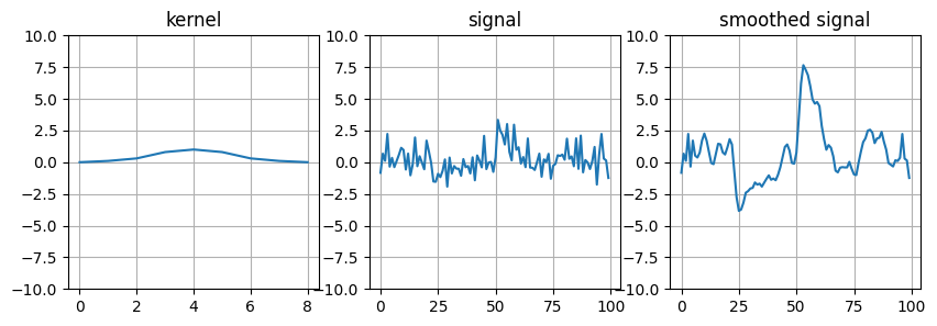 Next: [Matrices](matrices.html).